2.1 Deletion in Databases

2.1 Deletion in Databases#

Introduction#

You already know how to delete in SQL. Just use a DELETE FROM statement, and the rows you select are gone:

csc343h-dianeh=> select * from course;
 cnum |           name            | dept | breadth 
------+---------------------------+------+---------
| Intro to Databases        | CSC  | f
| Software Design           | CSC  | f
| Intro to Comp Sci         | CSC  | f
| Data Struct & Anal        | CSC  | f
| Intro to Visual Computing | CSC  | f
| Intro Archaeology         | ANT  | t
| Human Biol & Evol         | ANT  | f
| Organisms in Environ      | EEB  | f
| Marine Mammal Bio         | EEB  | f
| Compar Vert Anatomy       | EEB  | f
| Narrative                 | ENG  | t
| Rhetoric                  | ENG  | t
| The Graphic Novel         | ENG  | t
| Environmental Change      | ENV  | f
| Natl & Intl Env Policy    | ENV  | f
| Mediaeval Society         | HIS  | t
| Black Freedom             | HIS  | t
| COBOL programming         | CSC  | f
(18 rows)

csc343h-dianeh=> delete from course where name like '%COBOL%';
DELETE 1
csc343h-dianeh=> select * from course;
 cnum |           name            | dept | breadth 
------+---------------------------+------+---------
| Intro to Databases        | CSC  | f
| Software Design           | CSC  | f
| Intro to Comp Sci         | CSC  | f
| Data Struct & Anal        | CSC  | f
| Intro to Visual Computing | CSC  | f
| Intro Archaeology         | ANT  | t
| Human Biol & Evol         | ANT  | f
| Organisms in Environ      | EEB  | f
| Marine Mammal Bio         | EEB  | f
| Compar Vert Anatomy       | EEB  | f
| Narrative                 | ENG  | t
| Rhetoric                  | ENG  | t
| The Graphic Novel         | ENG  | t
| Environmental Change      | ENV  | f
| Natl & Intl Env Policy    | ENV  | f
| Mediaeval Society         | HIS  | t
| Black Freedom             | HIS  | t
(17 rows)

Let’s go under the hood to see what has to happen to make this occur. It’s a little more complicated than one might think.

Some background on storage#

First we need to think about how data is stored on a computer.

In order for a program to use data — to examine its value or perform operations on it — that data must be in memory. The variables used in a program, whether ints that take only a few bytes, or large data structures consuming a lot of space, are all stored in memory. However, a relational database is designed to be capable of handling data that is far too large to fit in memory all at once. What won’t fit in memory must be kept in secondary storage and brought into memory when it is needed.

Unfortunately, working in secondary storage (for example reading data from there or writing data to there) is orders of magnitude slower than working in memory.

Putting DBMSs aside for a moment, the slowness of file operations comes up even with very simple code such as this:

with open('data.txt', 'r') as f:
    one_line = f.readline()
    print(one_line)

When we ask to read a single line from the file and put it into the variable one_line, the operating system decides instead to read a big chunk of data (called called a “block” or “page”) and store it in a buffer in memory. In the long run, retrieving and storing a large block is very likely to save time. The next time the program asks for something from the file, there is a good chance it is already the buffer and so can be retrieved from there. Thus, a very slow file read is replaced by a very fast buffer read.

The OS manages multiple buffers and hides all these details from you; you can write a Python program that does file input and output without even knowing that buffering is going on.

On current systems, a block is typcially 4K, 8K, or 16K bytes.

How is a table stored?#

In postgreSQL, we see a table like this:

csc343h-dianeh=> select * from student;
  sid  | firstname |  surname   | campus |   email   | cgpa 
-------+-----------+------------+--------+-----------+------
 99132 | Avery     | Marchmount | StG    | avery@cs  | 3.13
 98000 | William   | Fairgrieve | StG    | will@cs   | 4.00
 99999 | Afsaneh   | Ali        | UTSC   | aali@cs   | 2.98
   157 | Leilani   | Lakemeyer  | UTM    | lani@cs   | 3.42
 11111 | Homer     | Simpson    | StG    | doh@gmail | 0.40
(5 rows)

Now we know our tables are kept in secondary storage much of the time. But how exactly is a table stored – what bytes go where? Is it laid out in row order, or column order? If in row order, is it sorted, and if so according to what column(s)?

And it turns out that more is stored than the data. PostgreSQL reveals this when we define a table.

csc343h-dianeh=> create table Student(
        sID integer primary key,
        firstName varchar(15) not null,
        surName varchar(15) not null,
        campus Campus,
        email varchar(25),
        cgpa CGPA);
CREATE TABLE
csc343h-dianeh=> d student
                     Table "university.student"
  Column   |         Type          | Collation | Nullable | Default 
-----------+-----------------------+-----------+----------+---------
 sid       | integer               |           | not null | 
 firstname | character varying(15) |           | not null | 
 surname   | character varying(15) |           | not null | 
 campus    | campus                |           |          | 
 email     | character varying(25) |           |          | 
 cgpa      | cgpa                  |           |          | 
Indexes:
    "student_pkey" PRIMARY KEY, btree (sid)

This last part holds important infomation:

Indexes:
    "student_pkey" PRIMARY KEY, btree (sid)

It says that postgreSQL has created an auxilliary data structure called an index. We didn’t ask for this structure, but postgreSQL made it on our behalf because we declared sID to be a primary key. This is a huge hint to the DBMS that we are probably going to use sID a lot to look things up in this table, and we are also probably going to do a lot of joins based on matching sIDs. The index data structure is designed to make those operations fast.

A database index#

An index is an extra structure that helps us find things quickly in our data. In the physical world, many books such as cookboos and textbooks typically have an index that maps topics to page numbers. If you want to bake macarons, you find “macaron” in the index and it tells you which pages contain macaron recipes. The index is organized alphabetically, to speed up search. The index is separate from the data itself (for example, the recipes). Without the index, to find macaron recipes or anything else, we would have to flip through the book one page at a time. A book can also have multiple indices, organized based on different things. For example, textbooks often have an author index and a topic index.

A database index is exactly analogous.

It is a separate structure from the data (the rows in our table).
It is organized to make search according to some attribute(s) (in this case, sID) fast.
When we find a desired sID in the index, stored with it is the location, in secondary storage, of the row for that sID. This location can be used as a pointer to go directly to that row.
Without the index, in order to find a desired sID, we would have to traverse through all the rows of the table.

When we created our Student table, postgreSQL told us:

Indexes:
    "student_pkey" PRIMARY KEY, btree (sid)

indicating that it made an index organized by the primary key we declared for the table, sID. We said that the index is organized to make search by sID fast. You learned in first year that a binary search tree is a good way to make search fast without compromising on fast insertion and deletion. We would want to upgrade to a balanced BST, in order to ensure O(log n) search time, where n is the number of values (in this case sIDs) in the tree. But even this is totally inadequate for our database index. If our data is so large that it can’t fit in memory, then our index, which must have one entry for each key value in the data, may not fit in memory either. But if a balanced BST index were stored in secondary storage, traversing it during a search would require bringing each node we visit into memory so that we could examine its value and decide whether to go left or right. Doing this very slow operation O(log n) times would take too much time.

Traversal would be faster if the search path were shorter, and we can make the search path shorter by making the tree wider. This is what a “B-tree” does — and notice that postgreSQL told us it had made a B-tree.

B-trees#

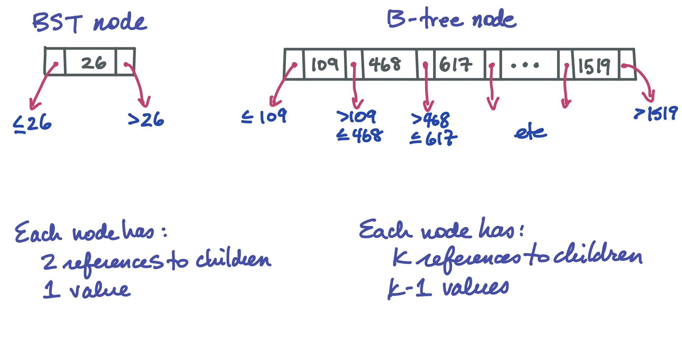
In a BST, a node has one value and two children. Choosing to go left or right in a balanced BST splits the search space roughly in half. In a B-tree, a node can hold up to k values and k+1 children, where k is some large number, perhaps 1024. Such a tree has a very large branching factor! This is what makes it wide and short, massively reducing the length of the search path and therefore the number of nodes that have to go through the very slow process of being brought into memory.

Here is how a B-tree node looks compared to a familiar BST node:

This is an outline of an entire B-tree:

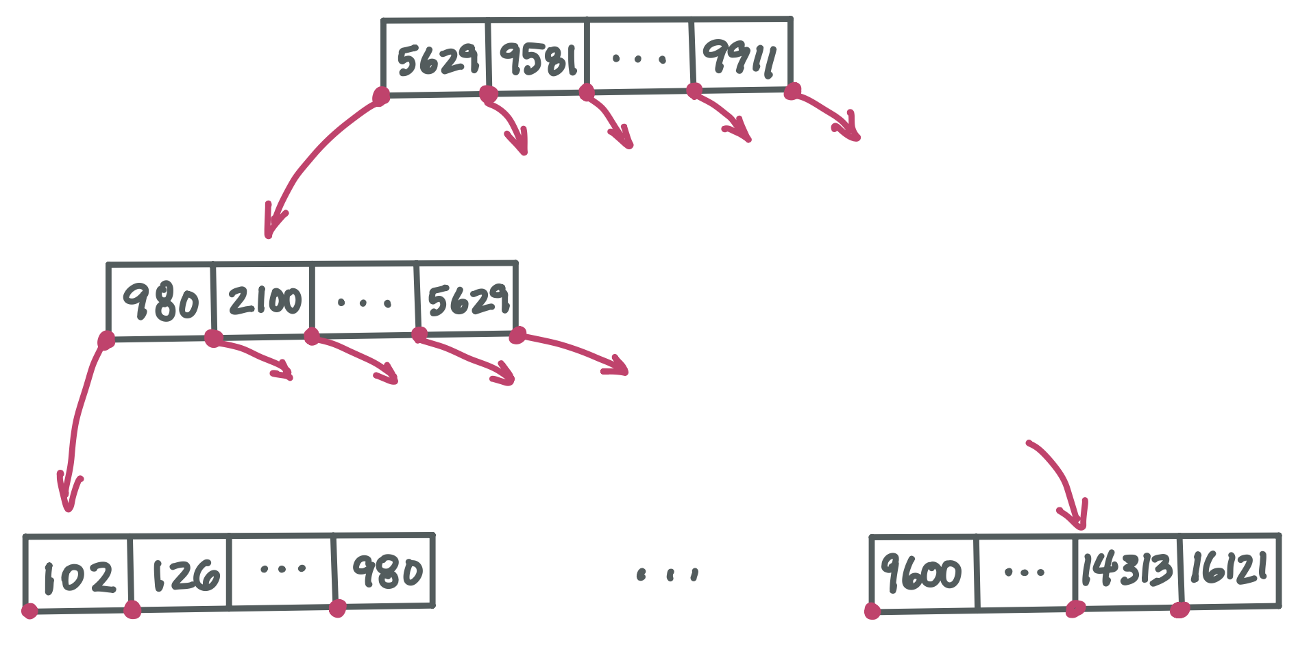
Note that although each pointer to a child node must be stored in its parent node, we aren’t showing the slots where these pointers would go. This is just to be more concise.

Because a B-tree node could have 1,024 children, it’s not practical to fully draw even a 2-level tree. Here we just show the path from root to leftmost child down the left side of the tree, plus the rightmost leaf. There would be many many more nodes if we drew this 3-level tree in full.

Notice that some values repeat in this example B-tree. For example, 980 appears in level two and then again in level three. Throughout this chapter, we are discussing a kind of B-tree that ensures every value occurs in a leaf node. In addition, some values will occur in nodes higher up as “sign post” that direct us to the leaf node containing the value we are searching for. (This is technically called a B+ tree).

How do we choose k?#

k is chosen so that the size of a node is the size of a block. This ensures that when we retrieve a block from secondary storage, it contains related data that is going to be useful.

The huge speed-up offered by a B-tree#

A BST node lets us choose to go left or right to continue our search for a desired value. But a B-tree node lets us choose between k+1 different child nodes, each corresponding to a range of values. This means that we divide the search space by roughly k each time we go down a level in the tree, rather than by just 2 as in a BST.

Suppose k is 1024. A huge branching factor like this means the tree is wide and short. For example, and using very round numbers:

Level 1 has 1 node and approximately 1,000 values
Level 2 has 1,000 nodes and approximately 1,000,000 values
Level 3 has 1,000,000 nodes and approximately 1,000,000,000 values

Having a short tree means the search path is short. This is really important, since, as we learned, each node on the search path must be brought into memory to look at it and moving a node (a block) into memory is slow.

Searching a B-tree is fast.

The leaves are different#

We’ve seen nodes with k values and k+1 child pointers. But of course a leaf doesn’t need child pointers. Instead, it stores k pointers that each go directly to the row of data for a given key.

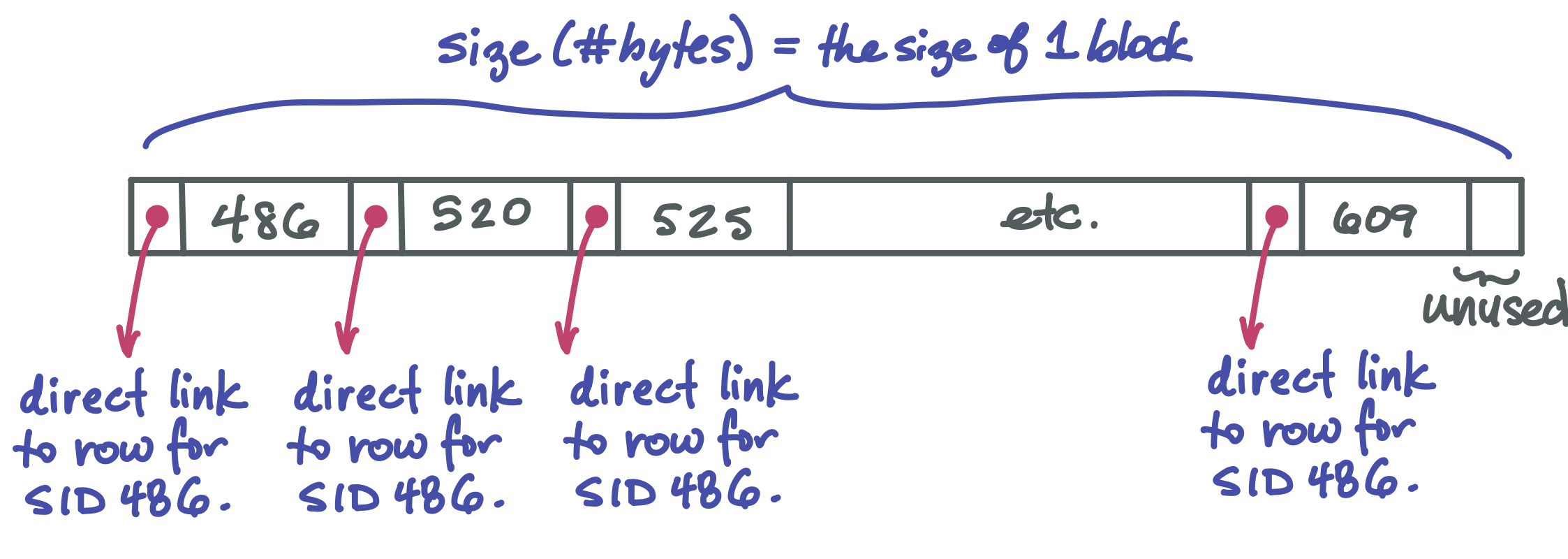
Each pointer in the B-tree is a “file pointers”, that is, an integer describing the number of bytes from the start of the file where an item is located.

The full picture: B-tree index plus data#

The B-tree nodes only store keys. When we search for a particular key in a B-tree, we end up at leaf that stores that key plus a direct file pointer to the row of the table for that key.

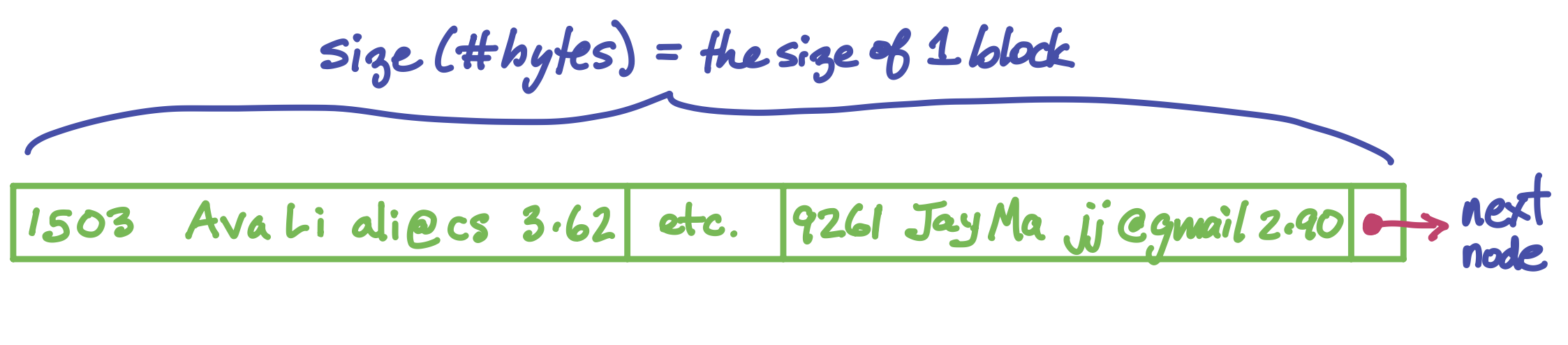
The data itself is a separate structure. One way it can be organized is as a linked list. (Of course the linked list is also in secondary storage, and each pointer from node to node is a file pointer). Each node of the linked list holds as many rows of the table as will fit into a block. It might look like this (but of course with much much more data in it):

Now we have all the pieces and are ready to see the full picture of how a SQL table can be stored:

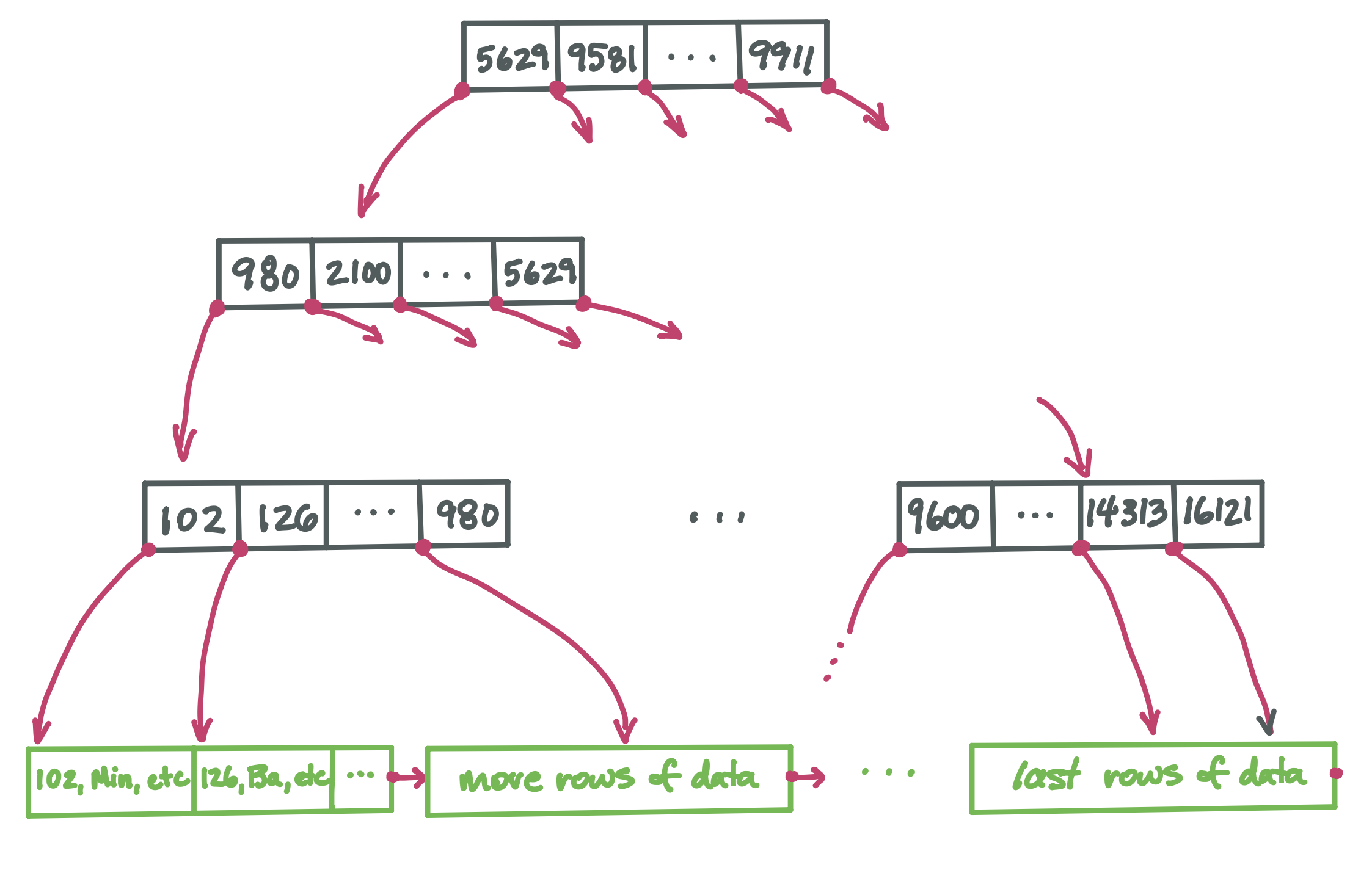
The black nodes form the index. It has a high branching factor, which makes the tree very short. This supports very fast search for any particular key. Every key appears in one leaf node (and possibly in some internal nodes too, helping direct us to the correct child node). Once we find the desired value in a leaf, we find with it a direct pointer to the row for that key value.

Deletion#

Now that we know how a table is stored, we are ready to talk about how deletion is implemented. This will be the topic of an upcoming lecture.