2.3 B-trees#
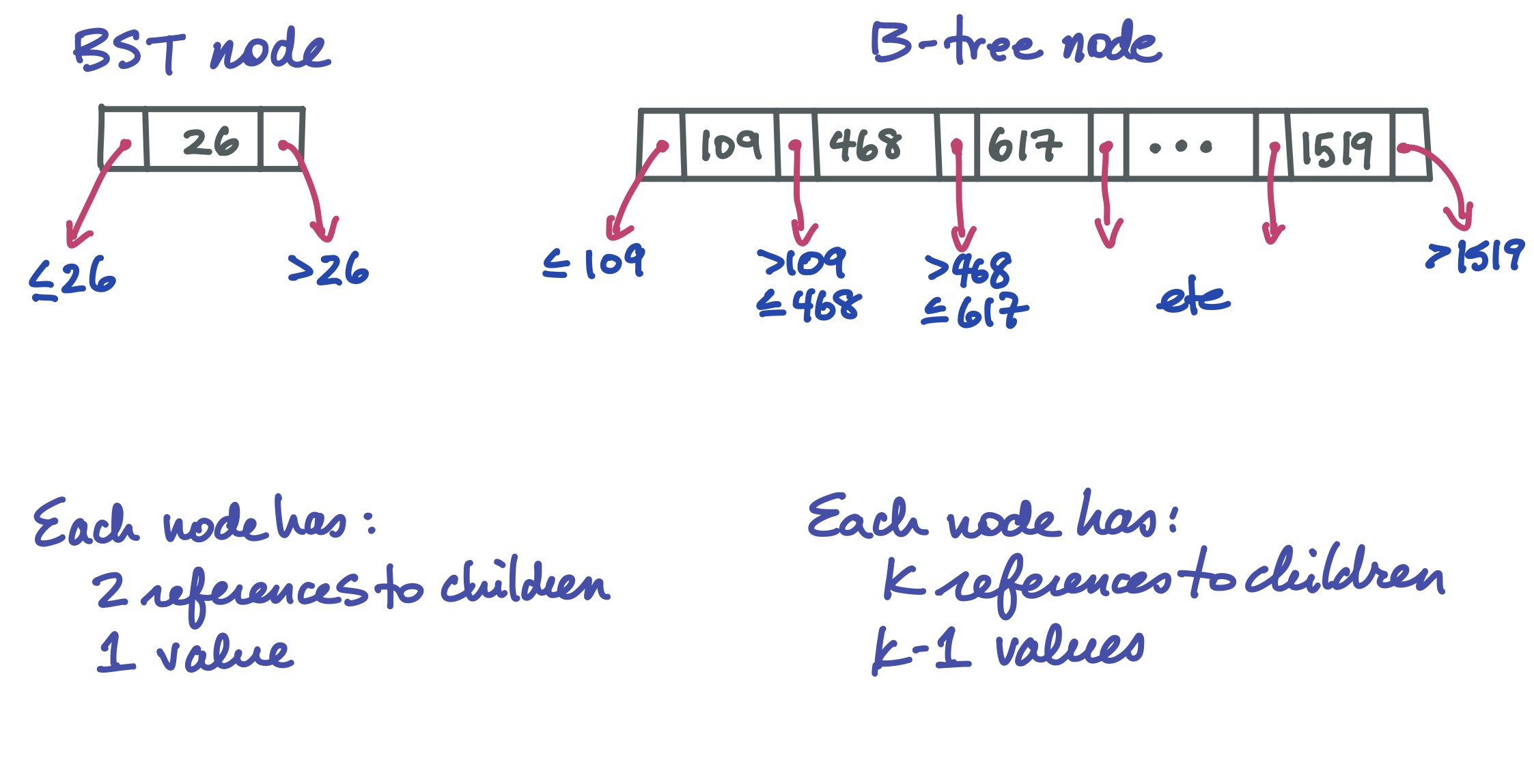
In a BST, a node has one value and two children. Choosing to go left or right in a balanced BST splits the search space roughly in half. In a B-tree, a node can hold up to k-1 values and k children, where k is some large number, perhaps 1,024. Such a tree has a very large branching factor! This is what makes it wide and short, massively reducing the length of the search path and therefore the number of nodes that have to go through the very slow process of being brought into memory.
Here is how a B-tree node looks compared to a familiar BST node:
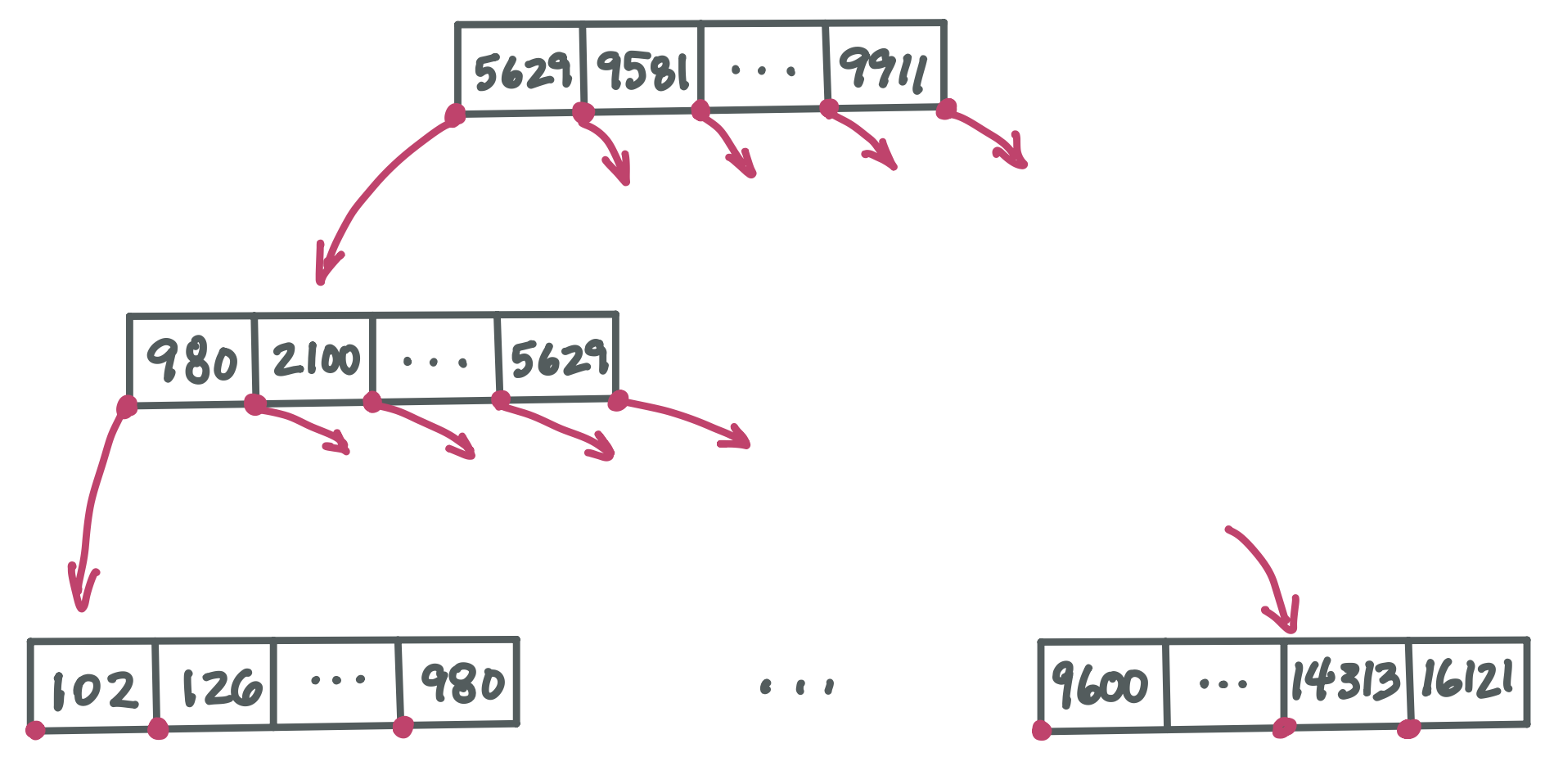
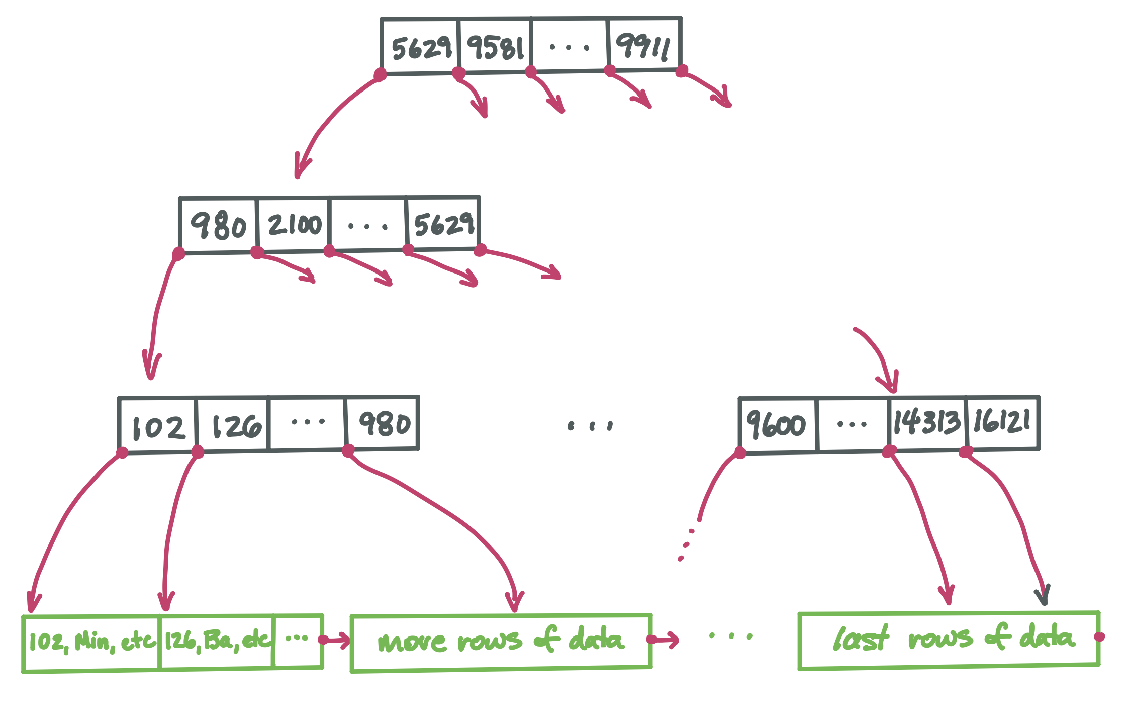
This is an outline of an entire B-tree:
Note that although each pointer to a child node must be stored in its parent node, we are no longer showing the slots where these pointers would go. This is just to be more concise.
Because a B-tree node could have 1,024 children, it’s not practical to fully draw even a 2-level tree. Here we just show the path from root to leftmost child down the left side of the tree, plus the rightmost leaf. There would be many many more nodes if we drew this 3-level tree in full.
Notice that some values repeat in this example B-tree. For example, 980 appears in level two and then again in level three. Throughout this chapter, we are discussing a kind of B-tree that ensures every value occurs in a leaf node. In addition, some values will occur in nodes higher up to help direct us to the leaf node containing the value we are searching for. (This is technically called a B+ tree).
How do we choose k?#
k is chosen so that the size of a node is the size of a block, or as close to that as we can get. This ensures that when we retrieve a block from secondary storage, it contains related data that is going to be useful.
The huge speed-up offered by a B-tree#
A BST node lets us choose to go left or right to continue our search for a desired value. But a B-tree node lets us choose between k different child nodes, each corresponding to a range of values. This means that we divide the search space by roughly k each time we go down a level in the tree, rather than by just 2 as in a BST.
Suppose k is 1,024. A huge branching factor like this means the tree is wide and short. For example, and using very round numbers:
Level 1 has 1 node and approximately 1,000 values
Level 2 has 1,000 nodes and approximately 1,000,000 values
Level 3 has 1,000,000 nodes and approximately 1,000,000,000 values
Having a short tree means the search path is short. This is really important, since, as we learned, each node on the search path must be brought into memory to look at it, and bringing a node (a block) into memory is slow.
B-tree search is fast!
The leaves are different#
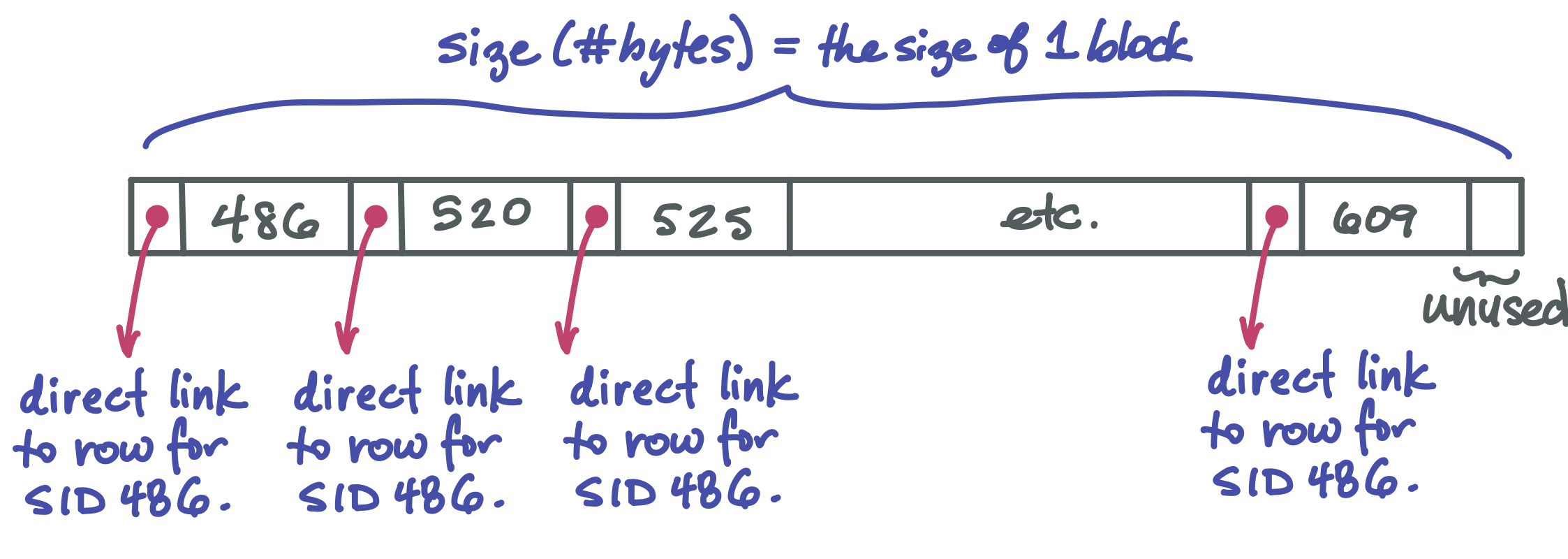
We’ve seen nodes with k-1 values and k child pointers. But of course a leaf doesn’t need child pointers. Instead, it stores k pointers that each go directly to the row of data for a given key.
Each pointer in the B-tree is a file pointer, that is, an integer describing the number of bytes from the start of a file where an item is located.
So where is the data?#
The B-tree nodes only store keys. When we search for and find a particular key in a B-tree, we end up at a leaf that stores that key plus a direct file pointer to the row of the table for that key.
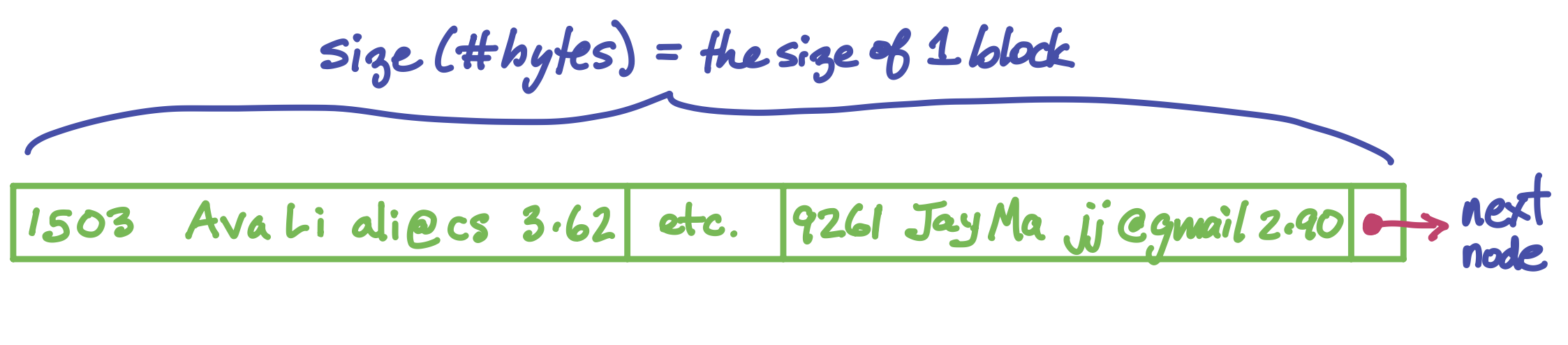
The data itself is in a separate structure. One way it can be organized is as a linked list. (Of course the linked list is also in secondary storage, and each pointer from node to node is a file pointer). Each node of the linked list holds as many rows of the table as will fit into a block. It might look like this (but of course with much much more data in it):
The full picture: B-tree index plus data#
Now we have all the pieces and are ready to see the full picture of how a SQL table can be stored:
The black nodes form the index. It has a high branching factor, which makes the tree very short. This supports very fast search for any particular key. Every key appears in one leaf node (and possibly in some internal nodes too, helping direct us to the correct child node). Once we find the desired value in a leaf, we find with it a direct pointer to the row for that key value.