Multi-Layer Perceptron
Learning Objectives
After reading this page, you should be able to:
- Describe the structure and components of a multi-layer perceptron.
- Trace the forward pass through hidden and output layers in matrix–vector form.
- Analyze the properties of the activation functions with respect to gradient-based training.
- Select output-layer activations suited to regression and classification tasks.
1 Introduction
On the previous page, Introducing the Neuron, we learned the computations performed by a single artificial neuron. We also saw that linear models, such as logistic and softmax regression, are equivalent to one-layer neural networks. Such a one-layer neural network has limited expressive power. It can only separate the input space with linear decision boundaries, so it cannot represent even simple non-linear patterns such as exclusive OR. One way forward is to use more neurons and to stack additional hidden layers between the input and the output. Each hidden layer computes new features from the features in the layer below it. Crucially, these features are learned rather than designed by hand. We never prescribe what each hidden neuron should mean.
This page makes that idea precise. It builds up to multi-layer perceptrons, which are neural networks with one or more hidden layers between the input and the output. We demonstrate how to choose inputs, targets, and layer sizes for the neural network by using handwritten digit recognition as a concrete design exercise. As with previous machine learning models, we assume the network has already been trained, so we can focus on inference, which means computing the network’s output for a given input. We write out these inference computations, also known as the forward pass, in matrix-vector form. Along the way, we introduce the notation in Table 2 used throughout the rest of the chapter. Finally, we survey four activation functions, examine how their properties affect gradient-based training, and discuss how to choose an activation function for each layer of a neural network.
2 Multi-Layer Perceptrons
Let us first recall the terms from Introducing the Neuron. An artificial neuron takes an input vector \(\mathbf{x}\) and computes a weighted sum of the inputs plus a bias, \(\mathbf{w}^\top \mathbf{x} + b\). This quantity is called the pre-activation. The neuron then passes the pre-activation through an activation function \(f\), which is typically non-linear, to produce its output \(y = f(\mathbf{w}^\top \mathbf{x} + b)\).
A neural network combines many neurons to represent complex non-linear functions. The neurons are arranged into layers, and the layers are stacked to form a network. The figure shown here is one example of a multi-layer perceptron.
Example of a Multi-Layer Perceptron
A multi-layer perceptron consists of three types of layers: an input layer, one or more hidden layers, and an output layer. Before describing each type, we need two terms for the nodes in these layers.
Definition: A unit is any node in a neural network. A neuron is a unit that computes its output from its inputs.
The input layer represents the input features to the model. Each input unit acts like a sensor that reports one measurement, such as the intensity of one pixel. It does not perform any computation and simply holds the data, so it is a unit but not a neuron.
Definition: A computational layer is a layer whose units are neurons.
The output layer is a computational layer and produces values that have a clear interpretation. For a classification task, the outputs typically represent a probability distribution over classes. For a regression task, the output is a continuous value.
Between the input and output layers are the hidden layers.
Definition: A hidden layer is any computational layer between the input layer and output layer.
The outputs of the hidden units are internal model representations rather than observed data or final predictions. Hidden units are essential for modelling complex, non-linear relationships.
A key structural property of this network is that it forms a directed acyclic graph (DAG). Such models are called feedforward neural networks.
Definition: A feedforward neural network is a neural network whose computation flows only from earlier layers to later layers, with no feedback loops.
Not every neural network is feedforward. Some networks contain loops, where a neuron’s output is fed back as input to itself or to an earlier layer. A loop lets the network carry information from one step to the next, which is useful for processing sequences such as text or audio. Networks with loops are called recurrent neural networks, and they are covered in more advanced courses such as Deep Learning.
We are now ready to define a multi-layer perceptron. An MLP is a particular kind of feedforward network, distinguished by how its layers are connected. So we first define a fully connected layer, the kind of layer shown throughout Figure 1.
Definition: A fully connected layer is a layer in which every unit receives input from every unit in the previous layer, and only from those units.
Definition: A multi-layer perceptron (MLP) is a feedforward neural network with one or more hidden layers between the input and output layers, in which every layer is fully connected.
The name carries some history. The perceptron, introduced by Frank Rosenblatt in 1958, was one of the earliest artificial neurons. It computed a weighted sum of its inputs and applied a hard threshold to make a binary decision, much like the threshold activation function we discuss later on this page. The term multi-layer perceptron has stuck for historical reasons, even though modern networks stack many such units and replace the original hard threshold with smooth activation functions.
When counting the number of layers in a multi-layer perceptron, we exclude the input layer because it does not perform any computation. Only computational layers, namely the hidden layers and the output layer, are counted. In this example, the network has two hidden layers and one output layer, so it is called a three-layer MLP.
Each neuron performs a simple, repeated computation similar to logistic regression. It takes inputs from the previous layer, computes a weighted sum with a bias, applies a non-linear activation function, and passes the result forward. By composing many such neurons across layers, an MLP can represent complex functions.
Let’s work through two examples to make these concepts more concrete. The exercise below shows a small neural network and asks you to answer several questions about the concepts introduced in this section.
Question: Answer the following questions about the network in Figure 2.
- How is the output of neuron \(D\) computed?
- How many neurons does the network have?
- How many layers does the network have?
- Is the network a feedforward neural network?
- Is every layer fully connected?
- Is the network a multi-layer perceptron?
A small feedforward network
Answer:
Neuron \(D\) receives two inputs, the value of input unit \(A\) and the output of neuron \(C\). Like any neuron, \(D\) computes a weighted sum of these two inputs, adds its bias, and passes the result through its activation function.
The network has 3 neurons, namely \(C\), \(D\), and \(E\). \(A\) and \(B\) are input units. They hold the input data and do not perform any computation.
The network has 3 layers. \(C\) is in the first layer because it receives only inputs. \(D\) is in the second layer because it depends on \(C\). \(E\) is in the third layer because it depends on \(D\). As before, we do not count the input layer.
Yes. Every edge points from an earlier layer to a later layer, and there are no loops.
No. The edge from \(A\) to \(D\) skips the first layer and connects the input layer directly to the second layer. In a fully connected layer, each unit receives input only from the units in the previous layer.
No. An MLP requires every layer to be fully connected, and this network is not.
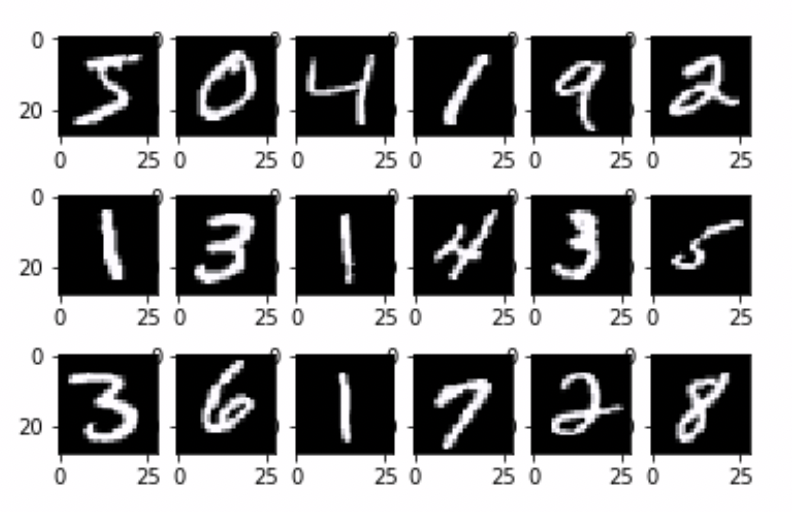
For the second example, let’s design an MLP for a familiar problem: handwritten digit recognition on the MNIST dataset. Recall from previous chapters that each example is a \(28 \times 28\) greyscale image of a handwritten digit, and each pixel stores an intensity value. The task is to classify each image as one of the 10 digits, 0 through 9. Designing an MLP for this task requires three decisions. We must decide how to represent the input, how to represent the target, and what the network structure should look like. The questions below walk through each decision.
MNIST handwritten digit samples
Answer:
We flatten each \(28 \times 28\) image into a vector \(\mathbf{x} \in \mathbb{R}^{784}\) and treat each pixel intensity as one input feature. The input layer has 784 units, one per pixel.
Answer:
There are 10 possible classes, one for each digit 0 through 9. We represent the target as a one-hot vector \(\mathbf{t} \in \mathbb{R}^{10}\). The entry at the position of the true digit is 1, and all other entries are 0. The first entry corresponds to the digit 0, so the target for the digit 3 has a 1 in its fourth entry.
\[\mathbf{t} = \begin{bmatrix} 0 & 0 & 0 & 1 & 0 & 0 & 0 & 0 & 0 & 0 \end{bmatrix}^\top\]
Answer:
The number of hidden layers and the number of units per layer are hyperparameters. They are design choices we make before training begins, so there is no single correct answer. For example, we might use 2 hidden layers, with 128 units in the first and 64 units in the second.
The output layer is determined by the task. For multi-class classification, the standard choice is a softmax layer with 10 units, one per class. The MLP then outputs a probability distribution over the 10 digits.
The hidden layers and the output layer play different roles. The hidden layers compute higher-level learned features from the input. The output layer converts these features into a classification outcome.
3 Inference in a 3-Layer MLP
Similar to how we learned about other machine learning models, we will discuss inference using an MLP before training an MLP. This section focuses on inference, where we use the learned weights and biases to compute the network’s output for a new input. On the next page, we will discuss training, in which we learn the weights and biases of an MLP from data using the backpropagation algorithm.
Let’s consider a 3-layer MLP and work through the process of computing its prediction for one input. We then compute the loss of this prediction, a step we will need for training. If you prefer, you can refer to Figure 1 as a concrete example.
3.1 Notation
A 3-layer MLP has 3 computational layers, which consist of 2 hidden layers and 1 output layer. We use a superscript \(^{(m)}\) to index each layer. The input layer is layer \(0\), the hidden layers are layers \(1\) and \(2\), and the output layer is layer \(3\).
For each layer \(m \in \{0, 1, 2, 3\}\), \(D^{(m)}\) denotes the number of units in that layer. For example, the MLP in Figure 1 has 3 input units (\(D^{(0)} = 3\)), 4 hidden units in each hidden layer (\(D^{(1)} = D^{(2)} = 4\)), and 2 output units (\(D^{(3)} = 2\)).
The input layer provides the input vector \(\mathbf{x} \in \mathbb{R}^{D^{(0)}}\) to the network, where \(x_k\) denotes the value of the \(k\)-th input unit. \[ \mathbf{x} = \begin{bmatrix} x_1 & x_2 & \cdots & x_{D^{(0)}} \end{bmatrix}^\top \]
Each computational layer then takes the previous layer’s activations as input and produces its own activations as output, which become the input to the next layer. We use \(\mathbf{h}^{(1)} \in \mathbb{R}^{D^{(1)}}\) and \(\mathbf{h}^{(2)} \in \mathbb{R}^{D^{(2)}}\) to denote the activations of layers 1 and 2, where \(h^{(m)}_j\) is the activation of unit \(j\) in layer \(m\). The letter \(h\) reminds us that these units are hidden. We use \(\mathbf{y} \in \mathbb{R}^{D^{(3)}}\) to denote the activations of layer 3, which is consistent with our previous notation for a model’s prediction output.
To compute its activations, each layer \(m \in \{1, 2, 3\}\) has its own weight matrix \(\mathbf{W}^{(m)} \in \mathbb{R}^{D^{(m)} \times D^{(m-1)}}\), bias vector \(\mathbf{b}^{(m)} \in \mathbb{R}^{D^{(m)}}\), and activation function \(f^{(m)}\). \(W^{(m)}_{j,k}\) denotes the weight from unit \(k\) in layer \(m-1\) to unit \(j\) in layer \(m\). The first subscript is the unit receiving the input, and the second subscript is the unit sending it. For example, \(W^{(1)}_{1,2}\) is the weight from input unit 2 to unit 1 in layer 1. \(b^{(m)}_j\) denotes the bias of unit \(j\) in layer \(m\). For the MLP in Figure 1, the weight matrices have the following shapes.
\[ \mathbf{W}^{(1)} \in \mathbb{R}^{4 \times 3}, \qquad \mathbf{W}^{(2)} \in \mathbb{R}^{4 \times 4}, \qquad \mathbf{W}^{(3)} \in \mathbb{R}^{2 \times 4} \]
Each layer \(m\) performs its computation in two steps. It first uses \(\mathbf{W}^{(m)}\) and \(\mathbf{b}^{(m)}\) to compute its pre-activations \(\mathbf{z}^{(m)} \in \mathbb{R}^{D^{(m)}}\), where \(z^{(m)}_j\) is the pre-activation of unit \(j\) in layer \(m\). It then applies \(f^{(m)}\) to \(\mathbf{z}^{(m)}\) to obtain its activations.
The hidden layers typically use a non-linear activation function. The output activation function \(f^{(3)}\) is chosen for the task, for example softmax for multi-class classification.
Table 1 summarizes the notation introduced so far.
| Symbol | Description |
|---|---|
| \(D^{(m)}\), \(m \in \{0, 1, 2, 3\}\) | Number of units in layer \(m\) |
| \(\mathbf{x} \in \mathbb{R}^{D^{(0)}}\) | Network input |
| \(\mathbf{h}^{(1)} \in \mathbb{R}^{D^{(1)}}\), \(\mathbf{h}^{(2)} \in \mathbb{R}^{D^{(2)}}\) | Activations of hidden layers 1 and 2 |
| \(\mathbf{y} \in \mathbb{R}^{D^{(3)}}\) | Network output |
| \(\mathbf{W}^{(m)} \in \mathbb{R}^{D^{(m)} \times D^{(m-1)}}\), \(m \in \{1, 2, 3\}\) | Weight matrix of layer \(m\) |
| \(\mathbf{b}^{(m)} \in \mathbb{R}^{D^{(m)}}\), \(m \in \{1, 2, 3\}\) | Bias vector of layer \(m\) |
| \(f^{(m)}\), \(m \in \{1, 2, 3\}\) | Activation function of layer \(m\) |
| \(\mathbf{z}^{(m)} \in \mathbb{R}^{D^{(m)}}\), \(m \in \{1, 2, 3\}\) | Pre-activations of layer \(m\) |
3.3 Output Layer Computations
Layer 3, the output layer, performs the same two steps with \(\mathbf{h}^{(2)}\) as its input. In Figure 1, the output \(\mathbf{y}\) has 2 entries. If the task is classification with two classes, \(f^{(3)}\) could be the softmax function, which turns these 2 entries into a probability distribution over the classes.
\[ \begin{aligned} \mathbf{z}^{(3)} &= \mathbf{W}^{(3)} \mathbf{h}^{(2)} + \mathbf{b}^{(3)} \\ \mathbf{y} &= f^{(3)} \left(\mathbf{z}^{(3)} \right) \end{aligned} \]
Unlike for the hidden layers, we write only the vectorized form for layer 3. The reason is that softmax is not applied element-wise, since each output \(y_j\) depends on the entire vector \(\mathbf{z}^{(3)}\). For regression with a single output, \(f^{(3)}\) is the identity and the output is the scalar \(y = z^{(3)}_1\). In short, the hidden layers use activation functions to build rich intermediate representations, while the output layer uses its activation function to produce a final prediction \(\mathbf{y}\) in a form that is meaningful for the task.
3.4 Computing the Loss
Inference ends once we have the prediction \(\mathbf{y}\). We go one step further and compute the loss of this prediction because training relies on it. Computing the loss requires a target, so this step applies only to examples whose targets are known, such as the training data.
Let \(\mathbf{t} \in \mathbb{R}^{D^{(3)}}\) denote the target vector, which has the same dimension as the network output \(\mathbf{y}\). For multi-class classification with \(K\) classes, \(\mathbf{t}\) is often a one-hot vector. For regression, \(t\) is usually a scalar. We still use the vector notation below so that the equations work for both cases. Let \(\mathcal{L}\) denote the loss for this example, which compares the output \(\mathbf{y}\) to the target \(\mathbf{t}\).
\[ \mathcal{L} = \mathcal{L} \left(\mathbf{y}, \mathbf{t} \right) \]
The specific form of \(\mathcal{L}\) depends on the task, for example squared error for regression or cross-entropy for classification. When we later train the network, we average this per-example loss over the whole dataset to obtain the cost \(\mathcal{E}\), and then minimize \(\mathcal{E}\) with gradient descent.
3.5 Putting Everything Together
Putting everything together, inference in a 3-layer MLP performs the following computations.
\[ \begin{aligned} \mathbf{z}^{(1)} &= \mathbf{W}^{(1)} \mathbf{x} + \mathbf{b}^{(1)}, & \mathbf{h}^{(1)} &= f^{(1)} \left(\mathbf{z}^{(1)} \right) \\ \mathbf{z}^{(2)} &= \mathbf{W}^{(2)} \mathbf{h}^{(1)} + \mathbf{b}^{(2)}, & \mathbf{h}^{(2)} &= f^{(2)} \left(\mathbf{z}^{(2)} \right) \\ \mathbf{z}^{(3)} &= \mathbf{W}^{(3)} \mathbf{h}^{(2)} + \mathbf{b}^{(3)}, & \mathbf{y} &= f^{(3)} \left(\mathbf{z}^{(3)} \right) \end{aligned} \]
These computations are called the forward pass because the computation flows forward from the input layer to the output layer. Inference is the task of computing a prediction, and the forward pass is the computation that performs it.
During training, we follow the forward pass with one more step that computes the loss.
\[ \mathcal{L} = \mathcal{L} \left(\mathbf{y}, \mathbf{t} \right) \]
The forward pass and the loss computation form the first stage of the backpropagation algorithm. Crucially, all of these computations are differentiable, which makes it possible to train the MLP with gradient-based optimization techniques. We will discuss the backpropagation algorithm in more detail in Backpropagation.
This notation works well for a 3-layer MLP, but it gives the input, the hidden layers, and the output different names (\(\mathbf{x}\), \(\mathbf{h}\), and \(\mathbf{y}\)). For an MLP with an arbitrary number of layers, it is more convenient to treat every layer in the same way. In the next section, we introduce a general notation that does this. The general notation can be especially helpful for visualizing the recursive nature of the Backpropagation algorithm.
4 Inference in a Multi-Layer Perceptron
We now generalize the notation from the previous section to write down the inference equations for an MLP with any number of layers. Table 2 collects the general notation for reference.
Generic multi-layer perceptron notation
The network has \(M\) computational layers. The layer index \(m\) runs from \(0\) to \(M\): \(m=0\) is the input layer, \(m=1,\dots,M-1\) are the hidden layers, and \(m=M\) is the output layer. As before, \(D^{(m)}\) denotes the number of units in layer \(m\).
The main change from the previous section is that we use one symbol \(\mathbf{a}^{(m)} \in \mathbb{R}^{D^{(m)}}\) to denote the activations of every layer \(m\), including the input \(\mathbf{a}^{(0)}\). The weight matrix \(\mathbf{W}^{(m)}\), bias vector \(\mathbf{b}^{(m)}\), activation function \(f^{(m)}\), and pre-activations \(\mathbf{z}^{(m)}\) are defined as before, now for \(m = 1, \ldots, M\). For the 3-layer MLP in the previous section, \(M = 3\), and the activations correspond to the earlier notation as follows.
\[ \mathbf{a}^{(0)} = \mathbf{x}, \qquad \mathbf{a}^{(1)} = \mathbf{h}^{(1)}, \qquad \mathbf{a}^{(2)} = \mathbf{h}^{(2)}, \qquad \mathbf{a}^{(3)} = \mathbf{y} \]
| Symbol | Description |
|---|---|
| \(M\) | Number of computational layers |
| \(m \in \{0, 1, \ldots, M\}\) | Layer index |
| \(D^{(m)}\) | Number of units in layer \(m\) |
| \(\mathbf{a}^{(0)}\) | Network input |
| \(\mathbf{W}^{(m)} \in \mathbb{R}^{D^{(m)} \times D^{(m-1)}}\) | Weight matrix of layer \(m\) |
| \(\mathbf{b}^{(m)} \in \mathbb{R}^{D^{(m)}}\) | Bias vector of layer \(m\) |
| \(f^{(m)}\) | Activation function of layer \(m\) |
| \(\mathbf{z}^{(m)} \in \mathbb{R}^{D^{(m)}}\) | Pre-activations of layer \(m\) |
| \(\mathbf{a}^{(m)} \in \mathbb{R}^{D^{(m)}}\) | Activations of layer \(m\) |
| \(\mathbf{t} \in \mathbb{R}^{D^{(M)}}\) | Target |
| \(\mathcal{L}(\mathbf{a}^{(M)}, \mathbf{t})\) | Loss for one example |
4.2 Output Layer Computations
The output layer (layer \(M\)) performs the same two steps, with its activation function \(f^{(M)}\) chosen for the task.
\[ \begin{aligned} \mathbf{z}^{(M)} &= \mathbf{W}^{(M)} \mathbf{a}^{(M-1)} + \mathbf{b}^{(M)} \\ \mathbf{a}^{(M)} &= f^{(M)} \left(\mathbf{z}^{(M)} \right) \end{aligned} \]
4.3 Computing the Loss
Inference ends with the prediction \(\mathbf{a}^{(M)}\). When the target \(\mathbf{t} \in \mathbb{R}^{D^{(M)}}\) is known, we compute the loss of this prediction for training.
\[ \mathcal{L} = \mathcal{L} \left(\mathbf{a}^{(M)}, \mathbf{t} \right) \]
The role of \(f^{(m)}\) raises an immediate question. What should each activation function be? The forward pass computations show that \(f^{(m)}\) is the only source of non-linearity in the entire computation. The next section examines the most common activation functions and the trade-offs among them.
5 Activation Functions
The activation function \(f\) is a crucial component of neural networks. It introduces non-linearity, which allows the network to learn complex patterns. Without non-linear activation functions, a multi-layer network would be equivalent to a single linear layer, regardless of how many layers it has.
Definition: An activation function \(f : \mathbb{R} \to \mathbb{R}\) is typically a non-linear scalar function. In an MLP, \(f\) is applied element-wise to a layer’s pre-activations \(\mathbf{z}^{(m)}\) to produce that layer’s activations \(\mathbf{a}^{(m)} = f \left(\mathbf{z}^{(m)} \right)\). The common choices are the threshold, sigmoid, \(\tanh\), and ReLU functions discussed below.
The one common exception is softmax, used in the output layer for multi-class classification. Softmax acts on the whole pre-activation vector at once rather than element-wise, but we still call it an activation function.
Four types of activation functions are commonly used in neural networks.
- Sigmoid
- Hyperbolic Tangent
- Rectified Linear Unit (ReLU)
- Threshold (Step Function)
These are simple activation functions, but it is still important to be able to analyze and understand their strengths and limitations. Modern neural networks (like large language models) now also use activation functions like GELU, Swish, and others, which are beyond the scope of these notes.
5.1 Sigmoid
The sigmoid function (also called the logistic function) is defined below.
\[\sigma(z) = \frac{1}{1 + e^{-z}}\]
Sigmoid activation function
We already encountered the sigmoid function in logistic regression. The sigmoid has two appealing properties as an activation function. First, it is a smooth and everywhere-differentiable approximation of the threshold (step) function, which makes gradient-based training possible. Second, it mirrors the biological intuition of a neuron firing. Instead of treating a neuron as either firing or not firing, we can interpret the sigmoid’s output as the neuron’s rate of firing, or the probability that it fires. This probabilistic interpretation is also why the sigmoid is commonly used in the output layer for binary classification.
In hidden layers, however, the sigmoid has three well-known drawbacks. All three concern how well gradient descent can train the network, similar to the problem we saw in Why Not Sigmoid with Squared Error?.
The first drawback is the dead neuron problem, which arises because the sigmoid’s derivative is close to zero for most inputs. A neuron is dead when gradient descent stops updating its incoming weights, because the derivative of its activation function is close to zero for the inputs it receives. The derivative of the sigmoid is
\[\sigma'(z) = \sigma(z)(1 - \sigma(z)),\]
which attains its maximum value of \(0.25\) at \(z = 0\) and approaches \(0\) as \(|z|\) grows. When a unit’s pre-activation is far from \(0\), the sigmoid is flat (saturated), so small changes to the unit’s incoming weights barely change its output. Gradient descent then barely updates these weights, and the unit stops learning, even if its output is wrong. This can happen in a network of any depth.
The second drawback is the vanishing gradient problem in deep networks. The gradients for the weights in early layers become smaller and smaller as the network gets deeper, so these weights learn very slowly or not at all. Since \(\sigma'(z)\) is at most \(0.25\), a change in the input always produces a smaller change in the output. By the chain rule, the derivative of the network’s output with respect to a weight in an early layer is a product with one \(\sigma'\) factor for every sigmoid layer between that weight and the output. Each factor is at most \(0.25\), so the product shrinks exponentially with depth.
The third drawback is that gradient descent cannot change a unit’s incoming weights in different directions, which slows down training. This happens because sigmoid activations are always positive. Suppose layer \(m\) uses the sigmoid. Then every input to a unit in layer \(m+1\) is positive, so increasing any of the unit’s incoming weights increases its pre-activation. Thus, each gradient descent update must either increase all of these weights or decrease all of them. If a good solution requires increasing some weights and decreasing others, gradient descent has to zigzag toward it.
Because of these drawbacks, the sigmoid is rarely used in the hidden layers of modern neural networks. We study it mainly for historical reference, since it was the standard choice in early neural networks and its drawbacks motivate the activation functions that replaced it.
5.2 Hyperbolic Tangent (tanh)
The hyperbolic tangent function is defined as
\[\tanh(z) = \frac{e^z - e^{-z}}{e^z + e^{-z}} = 2\sigma(2z) - 1.\]
The second equality shows that \(\tanh\) is just a rescaled and shifted sigmoid. We compress the sigmoid horizontally by a factor of \(2\), stretch it vertically by a factor of \(2\), and then shift it down by \(1\) so that it passes through the origin.
Tanh activation function
Because the two functions have similar shapes, \(\tanh\) inherits the sigmoid’s good property of being a smooth, everywhere-differentiable approximation of a step function. The key difference is that \(\tanh\) produces outputs in the range \((-1, 1)\) instead of \((0, 1)\).
As a result, \(\tanh\) fixes the third drawback of the sigmoid. Its activations are zero-centred, so they can be positive or negative. If layer \(m\) uses \(\tanh\), then the inputs to a unit in layer \(m+1\) can have different signs, so gradient descent can increase some of the unit’s incoming weights and decrease others in one update.
However, \(\tanh\) still suffers from the dead neuron problem. The derivative of \(\tanh\) is
\[\tanh'(z) = 1 - \tanh^2(z),\]
which approaches \(0\) as \(|z|\) grows. Just as with the sigmoid, this can lead to dead neurons.
Similarly, \(\tanh\) still suffers from the vanishing gradient problem because its derivative is less than \(1\) for every \(z \neq 0\). That said, the situation is slightly better than for the sigmoid. Since the maximum derivative of \(\tanh\) is four times that of the sigmoid, gradients shrink more slowly with depth.
Tanh is therefore an improvement over the sigmoid for hidden layers, but it is not a complete fix. We will see in the next subsection that ReLU avoids saturation on the positive side entirely.
5.3 Rectified Linear Unit (ReLU)
The Rectified Linear Unit (ReLU) is defined as
\[\text{ReLU}(z) = \max(0, z) = \begin{cases} z & \text{if } z \geq 0 \\ 0 & \text{if } z < 0. \end{cases}\]
In words, ReLU passes positive pre-activations through unchanged and clamps negative pre-activations to zero.
ReLU activation function
ReLU became the standard choice for hidden layers in the early 2010s, replacing the sigmoid and \(\tanh\). It remains a common default today, although many large models, such as large language models, use smoother variants like GELU. ReLU is cheap to compute, close to linear, and avoids the vanishing gradient problem. However, it still suffers from dead neurons.
ReLU is cheap to compute. The operation \(\max(0, z)\) requires only a comparison, so both the activation and its derivative are much cheaper to compute than the exponentials in the sigmoid and \(\tanh\).
ReLU is non-linear but close to linear. For positive inputs, ReLU is the identity and preserves the magnitude of the signal. As a result, ReLU networks behave almost like linear models in their active regions, which empirically makes them easier to optimize with gradient descent. The change in slope at \(z = 0\) is the only source of non-linearity, but it is enough to give the network its expressive power.
Most importantly, ReLU fixes the vanishing gradient problem. The derivative of ReLU is
\[\text{ReLU}'(z) = \begin{cases} 1 & \text{if } z > 0 \\ 0 & \text{if } z < 0. \end{cases}\]
ReLU is not differentiable at \(z = 0\), but in practice we define the derivative there to be \(0\) (or \(1\)), and this choice does not affect training. Unlike the sigmoid and \(\tanh\), ReLU does not flatten out for large positive inputs, so its derivative stays at \(1\) for any positive pre-activation. Gradients no longer shrink as they pass through ReLU layers. This is the main reason ReLU made it possible to train much deeper networks than before.
However, ReLU still suffers from the dead neuron problem, which is often called the dying ReLU problem in this context. Since the derivative of ReLU is exactly \(0\) for negative inputs, a unit whose pre-activation is negative for every training input always outputs \(0\), and gradient descent never updates its incoming weights. Variants such as Leaky ReLU and ELU (briefly mentioned in the next subsection) address this by allowing a small, non-zero output for negative pre-activations.
5.4 Threshold (Step Function)
The threshold function (also called the step function or Heaviside step function) is the simplest activation function. It is defined as
\[\sigma(z) = \begin{cases} 1 & \text{if } z \geq 0 \\ 0 & \text{if } z < 0. \end{cases}\]
In words, the threshold function outputs \(1\) when the pre-activation is non-negative and \(0\) otherwise. It is the original activation function used in perceptrons and most directly captures the “fires or does not fire” view of a biological neuron.
Threshold activation function
The threshold function cannot be used with gradient descent. Its derivative is \(0\) everywhere except at \(z = 0\), where it is undefined, so gradient descent never updates the weights. This is why the threshold function was replaced by smooth approximations like the sigmoid.
Today, the threshold function appears mainly in two contexts. It is the historical activation function of the perceptron, and it appears in pedagogical examples where the weights are picked by hand rather than learned from data.
5.5 Choosing an Activation Function
The choice of activation function is a hyperparameter to be chosen before training begins. In practice, the decision is made separately for the hidden layers and for the output layer.
For hidden layers, the activation function should be non-linear and support gradient-based training. Since hidden layers compute learned features rather than the final prediction, the choice is driven by how well the network trains. ReLU is a common default, with \(\tanh\) a reasonable alternative when zero-centred activations matter. The sigmoid is rarely used in hidden layers because of the drawbacks discussed above.
The activation function for the output layer is determined by the task. For regression, we often use the identity, which produces a real-valued prediction. For classification, we typically use the softmax function (as discussed in Softmax Regression), which produces a probability distribution over the classes.
6 Summary
A multi-layer perceptron is a feedforward neural network with one or more hidden layers between the input layer and the output layer. Hidden units compute learned intermediate features with no fixed meaning. Only the output layer produces task-specific predictions.
The forward pass starts from the input and repeats the same two steps at each computational layer. The layer first computes its pre-activations by multiplying the previous layer’s activations by a weight matrix and adding a bias vector. It then applies its activation function element-wise to obtain its own activations. The activations of the output layer form the network’s prediction, which the loss function compares to the target.
Non-linear activation functions in the hidden layers are essential. Without them, the network collapses into a single linear function. The choice of activation function relies heavily on whether it can improve gradient-based training, which relates to Fundamental Idea #1 (Learning is Optimization). The sigmoid suffers from dead neurons, vanishing gradients in deep networks, and all-positive activations. Tanh fixes the last drawback, and ReLU avoids vanishing gradients, which makes ReLU a common default for hidden layers. The activation function of the output layer is chosen by the task. We use the identity for regression and the softmax for classification.
This page covered inference with known parameters. The next page, Expressiveness of Neural Networks, examines which functions neural networks can represent. Backpropagation then addresses learning the parameters of an MLP.