In this chapter, we’re going to explore a topic that is at once new
and familiar: sorting a list. By this point in the course, you’ve used
Python’s built-in functions sorted and
list.sort to sort lists to help solve various programming
problems. But you might wonder, how do these functions work, and how
efficient are they?
Over the past few chapters, we’ve explored various ways of organizing
data into data structures like linked lists, trees, and graphs, and
learned how to implement various common operations on those data
structures. This chapter is going to be a little different. We’re going
to look at just one data structure, the Python array-based
list, and one operation, sorting it. The complexity that
we’ll learn about stems from the fact that there are many different
algorithms for sorting a list, that differ not just in individual lines
of code but in their conceptual approach.
In this chapter, we’ll learn about a diverse range of sorting algorithms, covering their ideas, their implementations, and their running times. By the end of this chapter, we hope that you appreciate just how inventive computer scientists can be when designing new algorithms, and how there can be vastly different ways of solving the same problem.
A little motivation: binary search
Before getting to our search algorithms, we’ll take a quick stop at one topic that both motivates why sorting a list can be useful, and previews some of the technical loop designs we’ll start using when we get to the sorting algorithms in the next section. This topic is binary search, which we touched on back in 15.5 Introduction to Binary Search Trees.
Recall the standard way of searching for an item in a list, using a for loop with an early return:
def search(lst: list, item: Any) -> int:
    """Return whether item appears in this list."""
    for element in lst:
        if element == item:
            return True

    return False
This function has a worst-case running time of \(\Theta(n)\), where \(n\) is the length of lst.
Intuitively, there are cases where the for loop will need to iterate
\(n\) times, checking each element of
the list against the item being searched for. After all, any of these
elements might be the desired item!
We said back in Section 15.5 that if
we have a sorted list, then we don’t need to check all of its
elements if we’re smart about which elements we’re checking. To see why,
suppose we have a sorted list lst containing one million
numbers, and we’re searching for the number 111. If we check the middle
element (the one at index 500,000), there are three
possibilities: Unsurprisingly, these match up exactly with various
cases of BinarySearchTree.__contains__!
- If 111 is equal to
lst[500000], then we’ve found the item and can returnTrue. - If 111 is less than
lst[500000], then we know it must appear in the left half of the list, because the list is sorted. We can ignore all elements with index>= 500000. - If 111 is greater than
lst[500000], then we know it must appear in the right half of the list, again because the list is sorted. We can ignore all elements with index< 500000.
In the latter two cases, a single comparison allows us to ignore roughly half of the list’s items. And we can repeat this process on either the left or right half of the list until we’ve either found the item or ended with no more list elements to check. This algorithm is known as binary search, where the “binary” refers to the fact that at every comparison, the range of elements to check is halved.
Now, you might be expecting us to implement binary search
recursively, and indeed this is possible, following the same approach as
BinarySearchTree.__contains__. However, we’re going to
implement it iteratively instead, to prepare us for the more complex
iterative sorting algorithms you’ll study in the next two sections.
Implementing binary search
The key idea for implementing binary search iteratively is that we
need to keep track of the current search range, which gets
smaller every time a new item is checked. To do this, we’ll use two
variables, b and e, to represent the endpoints
of this range: at any point in time in our algorithm, the current search
range is the list slice lst[b:e]. These variables will
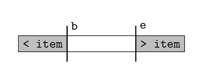
divide our list into three parts:
lst[0:b]contains only items that are known to be less than the item being searched for.lst[b:e]is the current search range; we don’t know whether the items in here are less than, equal to, or greater than the item being searched for.lst[e:len(lst)]contains only items that are known to be greater than the item being searched for.
Here is how we’ll start our implementation:
def binary_search(lst: list, item: Any) -> bool:
    """Return whether item is in lst using the binary search algorithm.

    Preconditions:
        - lst is sorted in non-decreasing order
    """
    b = 0
    e = len(lst)
So at the start of our search, the full list
(lst[0:len(lst)]) is being searched. Now, the binary search
algorithm uses a while loop to decrease the size of the
range.
First, we calculate the midpoint
mof the current range.Then we compare
lst[m]againstitem.- If
item == lst[m], we can returnTrueright away. - If
item < lst[m], we know that all indexes>= mcontain elements larger thanitem, and so updateeto reflect this. - If
item > lst[m], we know that all indexes<= mcontain elements less than theitem, and so updatebto reflect this.
- If
Let’s write out our loop:
def binary_search(lst: list, item: Any) -> bool:
    """Return whether item is in lst using the binary search algorithm.

    Preconditions:
        - lst is sorted in non-decreasing order
    """
    b = 0
    e = len(lst)

    while ...:
        m = (b + e) // 2
        if item == lst[m]:
            return True
        elif item < lst[m]:
            e = m
        else:  # item > lst[m]
            b = m + 1
Finally, to complete the loop condition, we can take our usual
indirect approach and ask, when should the loop stop? Intuitively, this
is when there are no more items to check—when lst[b:e] is
empty. This occurs when b >= e, and negating this gives
us our loop condition.
def binary_search(lst: list, item: Any) -> bool:
    """Return whether item is in lst using the binary search algorithm.

    Preconditions:
        - lst is sorted in non-decreasing order
    """
    b = 0
    e = len(lst)

    while b < e:
        m = (b + e) // 2
        if item == lst[m]:
            return True
        elif item < lst[m]:
            e = m
        else:  # item > lst[m]
            b = m + 1

    # If the loop ends without finding the item, the item is not in the list.
    return False
Don’t forgot about loop invariants!
Because while loops have less explicit structure than for loops, it can be easy to get lost in what the code is doing. Adding good loop invariants is a great way of helping us track what while loops are doing, and we’ll be using this technique throughout this chapter.
In our final version of binary_search below, we’ve added
two loop invariants to encode how b and e
split up the list.
def binary_search(lst: list, item: Any) -> bool:
    """Return whether item is in lst using the binary search algorithm.

    Preconditions:
        - lst is sorted in non-decreasing order
    """
    b = 0
    e = len(lst)

    while b < e:
        # Loop invariants
        assert all(lst[i] < item for i in range(0, b))
        assert all(lst[i] > item for i in range(e, len(lst)))

        m = (b + e) // 2
        if item == lst[m]:
            return True
        elif item < lst[m]:
            e = m
        else:  # item > lst[m]
            b = m + 1

    # If the loop ends without finding the item, the item is not in the list.
    return False
Running-time analysis
Now that we’ve completed our implementation of
binary_search, let’s talk about running time. We claimed at
the start of this section that binary search is faster than searching
every item in the list—is it?
We won’t do a formal analysis here, but this is the main idea. Our
implementation has two loop variables, b and e
that change over time in unpredictable ways, depending on the result of
comparing item and lst[m] at each iteration.
However, it we focus on the quantity e - b, we can make the
following observations:
e - binitially equals \(n\) the length of the input list.- The loop stops when
e - b <= 0. - At each iteration,
e - bdecreases by at least a factor of 2. This is the part that requires a formal proof, using the definition ofmand cases that match the if statement in the code.
So putting these three observations together, we get that
binary_search runs for at most \(1 + \log_2 n\) iterations, with each
iteration taking constant time. Since the other statements outside of
the loop are constant time, the worst-case running time is \(\cO(\log n)\). Much better indeed than the
linear search’s \(\Theta(n)\) running
time for unsorted lists.
So for large datasets where we plan to do many search operations, it is often more efficient to pre-sort the list of data so that every subsequent search runs quickly. As for how we actually do that sorting—stay tuned for the next section!