In the next part of this chapter, we’re going to learn about one particular application of trees for storing data called the binary search tree. This new data structure forms the basis of more advanced tree-based data structures you’ll learn about in future courses like CSC263/265.
The Multiset abstract data type
To start, let’s introduce one new abstract data type that is an extension of the Set ADT that allows for duplicates:
Multiset
- Data: an unordered collection of values, allowing duplicates
- Operations: get size, insert a value, remove one occurrence of a specified value, check membership in the multiset.
You might be imagining a few different possible implementations for
the Multiset ADT already using familiar Python data types like
list and dict. Let’s briefly consider two
possible implementations the Multiset ADT.
Implementing Multiset
using list and Tree
Suppose we use a list to implement the Multiset ADT,
where we simply append new items to the end of the list. As we discussed
all the way back in Chapter
9, this implementation would make searching for a
particular item a \(\Theta(n)\)
operation, proportional to the size of the collection.
If we used a Tree instead of a list, we’d
get the same behaviour: if the item is not in the tree, every item in
the tree must be checked. So just switching from lists to trees isn’t
enough to do better!
However, one of the great insights in computer science is that adding some additional structure to the input data can enable new, more efficient algorithms. You have seen a simple form of this called augmentation in previous exercises, and in this section we’ll look at more complex “structures”.
In the case of Python lists, if we assume that the list is
sorted, then we can use the binary search
algorithm to improve the efficiency of searching to \(\Theta(\log
n)\). We haven’t yet formally covered binary search, though
we’ll see it later in the course. If you’re curious we’ve put in some
reference videos from CSC108 at the bottom of this section. But
though ensuring the list is sorted does make searching faster, the same
limitations of array-based lists apply: insertion and deletion into the
front of the list takes \(\Theta(n)\).
So the question is: can we achieve efficient (faster than linear)
search, insertion, and deletion implementations all at once? Yes we
can! Now, you might be recalling that Python’s
set and dict already have constant-time
search, insertion, and deletion! It is indeed possible to implement the
Multiset ADT efficiently using a dict (keeping track of
duplicates in a “smart” way). But we’re going to explore a different
approach this chapter that allows for other efficient operations as
well.
Binary search trees: definitions
To implement the Multiset ADT efficiently, we will combine the branching structure of trees with the idea of binary search to develop a notion of a “sorted tree”.
First, some definitions. A binary tree is a tree in which every item has two (possibly empty) subtrees, which are labelled its left and right subtrees. An item in a binary tree satisfies the binary search tree property when its value is greater than or equal to all items in its left subtree, and less than or equal to all items in its right subtree. Note that duplicates of the root are allowed in either subtree in this version.
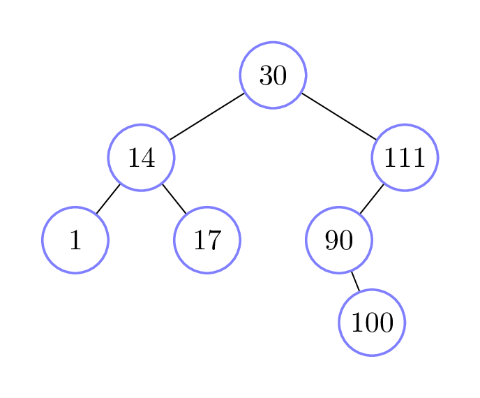
A binary tree is a binary search tree (BST) when every item in the tree satisfies the binary search tree property (the “every” is important: for an arbitrary binary tree, it’s possible that some items satisfy this property but others don’t). An example of a binary search tree is shown on the right.
We can think of binary search trees as a “sorted tree”: even if the data isn’t inserted in sorted order, the BST keeps track of it in a sorted fashion. This makes BSTs extremely efficient in doing operations like searching for an item; but unlike sorted Python lists, they can be much more efficient at insertion and deletion while maintaining the sortedness of the data!
Representing a binary search tree in Python
We’ll define a new class BinarySearchTree to represent
this form of tree. This class is based on the Tree class we
studied, but with a few important differences. First, because we know
there are only two subtrees, and the left/right ordering matters, we use
explicit attributes to refer to the left and right
subtrees: So we’ve replaced the Tree
_subtrees attribute with two new attributes,
_left and _right.
class BinarySearchTree:
    """Binary Search Tree class.
    """
    # Private Instance Attributes:
    #   - _root:
    #       The item stored at the root of this tree, or None if this tree is empty.
    #   - _left:
    #       The left subtree, or None if this tree is empty.
    #   - _right:
    #       The right subtree, or None if this tree is empty.
    _root: Optional[Any]
    _left: Optional[BinarySearchTree]
    _right: Optional[BinarySearchTree]
Another difference between BinarySearchTree and
Tree how we distinguish between empty and non-empty trees.
In the Tree class, an empty tree has a _root
value of None, and an empty list []
for its list of subtrees. In the BinarySearchTree class, an
empty tree also has a _root value of None, but
its _left and _right attributes are set to
None as well. Moreover, for BinarySearchTree,
an empty tree is the only case where any of the attributes can
be None; when we represent a non-empty tree, we do so by
storing the root item (which isn’t None) at the root, and
storing BinarySearchTree objects in the _left
and _right attributes. The attributes _left
and _right might refer to empty binary search
trees, but this is different from them being
None! This is also what we did for
RecursiveList back in Section
14.5. We document these as representation invariants for
BinarySearchTree, which are Python translations of
“self._root is None if and only if
self._left is None” and “self._root is None if
and only if self._right is None”.
class BinarySearchTree:
    """Binary Search Tree class.

    Representation Invariants:
      - (self._root is None) == (self._left is None)
      - (self._root is None) == (self._right is None)
    """
And finally, we add one more English representation invariant for the
BST property itself. Here is our full BinarySearchTree
class header, docstring, and instance attributes:
class BinarySearchTree:
    """Binary Search Tree class.

    Representation Invariants:
      - (self._root is None) == (self._left is None)
      - (self._root is None) == (self._right is None)
      - (BST Property) if self._root is not None, then
          all items in self._left are <= self._root, and
          all items in self._right are >= self._root
    """
    # Private Instance Attributes:
    #   - _root:
    #       The item stored at the root of this tree, or None if this tree is empty.
    #   - _left:
    #       The left subtree, or None if this tree is empty.
    #   - _right:
    #       The right subtree, or None if this tree is empty.
    _root: Optional[Any]
    _left: Optional[BinarySearchTree]
    _right: Optional[BinarySearchTree]
And here are the initializer and is_empty methods for
this class, which are based on the corresponding methods for the
Tree class:
class BinarySearchTree:

    def __init__(self, root: Optional[Any]) -> None:
        """Initialize a new BST containing only the given root value.

        If <root> is None, initialize an empty BST.
        """
        if root is None:
            self._root = None
            self._left = None
            self._right = None
        else:
            self._root = root
            self._left = BinarySearchTree(None)   # self._left is an empty BST
            self._right = BinarySearchTree(None)  # self._right is an empty BST

    def is_empty(self) -> bool:
        """Return whether this BST is empty.
        """
        return self._root is None
Note that we do not allow client code to pass in left and right subtrees as parameters to the initializer. This is because binary search trees have a much stronger restriction on where values can be located in the tree, and so a separate method is used to insert new values into the tree that will ensure the BST property is always satisfied.
But before we get to the BST mutating methods (inserting and deleting items), we’ll finish this section by studying the most important non-mutating BST method: searching for an item.
Searching a binary search tree
For general trees, the standard search algorithm is to compare the
item against the root, and then recursively search in each
of the subtrees until either the item is found, or all the subtrees have
been searched. When item is not in the tree, every item
must be searched.
In stark contrast, for BSTs the initial comparison to the root tells you which subtree you need to check. For example, suppose we’re searching for the number 111 in a BST. We check the root of the BST, which is 50. Since 111 is greater than 50, we know that if it does appear in the BST, it must appear in the right subtree, and so that’s the only subtree we need to recurse on. On the other hand, if the root of the BST were 9000, then we would need to recurse on the left subtree, since 111 is less than 9000.
That is, in the recursive step for
BinarySearchTree.__contains__, only one recursive call
needs to be made, rather than two!
class BinarySearchTree:
    def __contains__(self, item: Any) -> bool:
        """Return whether <item> is in this BST.
        """
        if self.is_empty():
            return False
        else:
            if item == self._root:
                return True
            elif item < self._root:
                return self._left.__contains__(item)
            else:
                return self._right.__contains__(item)
While this code structure closely matches the recursive code template
for the general Tree class, we can also combine the two
levels of nested ifs to get a slightly more concise version:
class BinarySearchTree:
    def __contains__(self, item: Any) -> bool:
        """Return whether <item> is in this BST.
        """
        if self.is_empty():
            return False
        elif item == self._root:
            return True
        elif item < self._root:
            return self._left.__contains__(item)
        else:
            return self._right.__contains__(item)