Now we return to the reason we started talking about binary search
trees in the first place: we wanted a more efficient implementation of
the Multiset ADT, which supports search, insertion, and deletion. The
three BinarySearchTree methods __contains__,
insert, and remove all have the same recursive
structure, and their running times are very similar. We’ll focus on
analyzing BinarySearchTree.__contains__ here.
class BinarySearchTree:
    def __contains__(self, item: Any) -> bool:
        """Return whether <item> is in this BST.
        """
        if self.is_empty():
            return False
        elif item == self._root:
            return True
        elif item < self._root:
            return self._left.__contains__(item)  # or, item in self._left
        else:
            return self._right.__contains__(item)  # or, item in self._right
Running-time
analysis of BinarySearchTree.__contains__
Because BinarySearchTree.__contains__ is recursive,
we’ll use the same approach for analyzing its runtime as we did with
Tree methods in 15.4
Running-Time Analysis for Tree Operations.
We’ll start with analyzing the non-recursive running time of the
method, because that’s quite simple in this case. In fact, if we assume
that each recursive call takes constant time, then the body runs in
constant time, since the self.is_empty(),
item == self._root, and item < self._root
checks and return statements each take constant time! So this is quite a
bit simpler than Tree.__len__: here we count the
non-recursive cost as 1 step per recursive call.
What about the recursive call structure for this method? Unlike
Tree.__len__, BinarySearchTree.__contains__
only recurses on one subtree rather than all
subtrees.Of course, this is made possible by using the BST
property to decide which subtree to recurse into. This means that
our recursive call diagram is a bit different than the one we looked at
for Tree.__len__. Intuitively, each recursive call that is
made goes down one level into the BST. For example, suppose we
search for the item 99 in the following binary search tree:
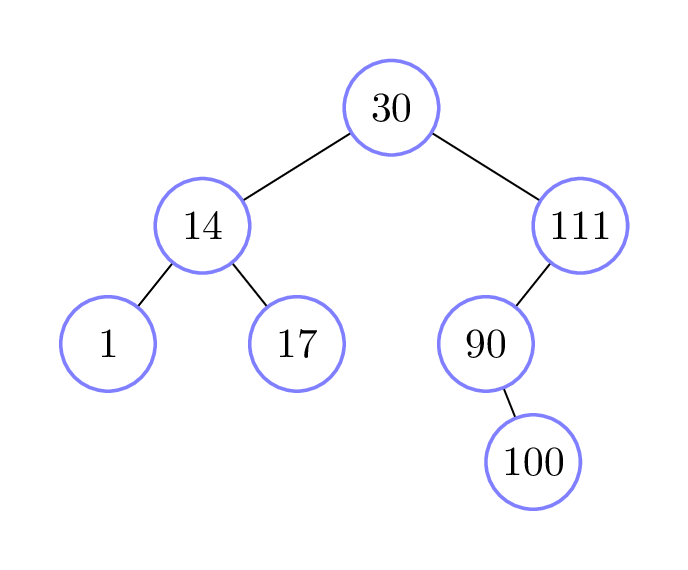
In this case, five calls to
BinarySearchTree.__contains__ are made in total:
- The initial call recurses on the right subtree, since \(99 > 30\).
- The second call recurses on the left subtree, since \(99 < 111\).
- The third call recurses on the right subtree, since \(99 > 90\).
- The fourth call recurses on the left subtree, since \(99 < 100\).
- Finally, the fifth call is on an empty tree, and so returns
Falsewithout making any more recursive calls.
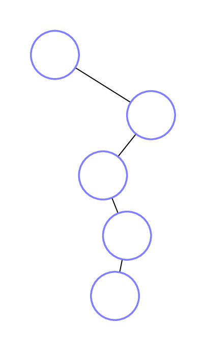
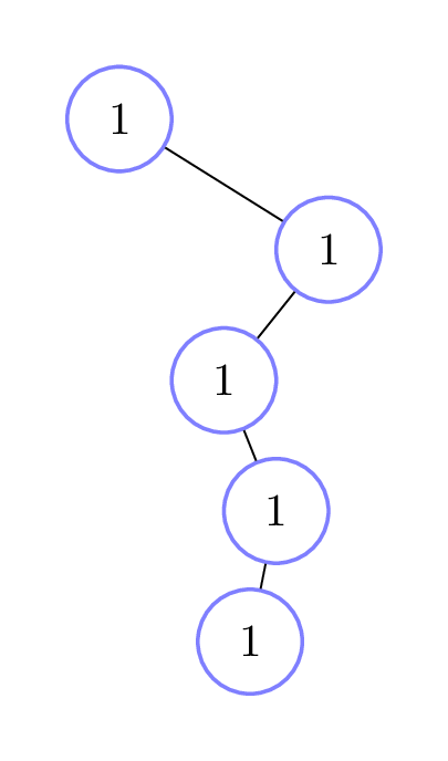
Here is the recursive call diagram for this example; we’ve kept the left-right structure to help you visualize what’s going on. The diagram on the left shows just the recursive call structure, while the one on the right fills in each node with the non-recursive running time of that call, which is simply 1 step in this case.
But as you might expect, the number of recursive calls differs
depending on the values stored in the tree and the values being searched
for. For example, if we took the above tree and searched instead for 30,
then only one call to BinarySearchTree.__contains__ is made
(the original one), since the item being searched for is equal to the
root of the tree.
So BinarySearchTree.__contains__ has a spread of running
times, and as usual we will focus on the worst-case running time. We
won’t do a formal analysis here, but the intuition is that the total
number of recursive calls is at most the height of the BST plus
1, since the longest possible “search path” for an item is equal to the
height of the BST, plus 1 for recursing into an empty
subtree. Our above example diagram illustrates this “height
plus 1” running time. What other numbers could we have searched for that
would have led to this running time? And since each call has a
non-recursive running time of 1 step, this gives us a total of \(h + 1\) steps, where \(h\) is the height of the BST. So the
worst-case running time for BinarySearchTree.__contains__
is \(\Theta(h)\). The same analysis
holds for the insert and remove methods as
well. Note that the remove method is a bit more
complicated to analyze, since it makes use of some helper methods.
However, we can use the same ideas to show that these helper methods
have a worst-case running time of \(\Theta(h)\).
Binary search tree height vs. size
You might look at \(\Theta(h)\) and recall that we said searching through an unsorted list takes \(\Theta(n)\) time, where \(n\) is the size of the list. Since both of these Theta expressions look linear, it might seem that BSTs are no faster than unsorted lists for implementing the Multiset ADT.
This is where our choice of variables really matters. While it is true that the worst-case running time for BST search is proportional to the BST’s height, in general the height of a BST can be much smaller than its size!
In fact, if we consider a BST with \(n\) items, its height can be as large as \(n\) (in this case, the BST just looks like a list). However, it can be as small as \(\log_2 n\)! Why? Because of the following theorem.We won’t prove this theorem here, but it is possible to prove it using induction!
Let \(B\) be a binary search tree with height \(h\) and size \(n\). Then \(n \leq 2^h - 1\). (Or equivalently, \(h \geq \log_2(n + 1)\).)
So if we can guarantee that binary search trees always have
height roughly \(\log_2 n\), then in
fact all three BST operations (search, insert, delete) have a worst-case
running time of \(\Theta(h) = \Theta(\log
n)\). Much better than either lists or Trees!
Looking ahead
The preceding paragraph sounds great, but it relies on a big assumption: that the height of a binary search tree will always be roughly \(\log_2 n\). Unfortunately, the insertion and deletion algorithms we have studied in this chapter do not guarantee this property holds when we mutate a binary search tree.One example is when you insert items into a binary search tree in sorted order.
However, computer scientists have developed more sophisticated insertion and deletion algorithms which do ensure that the height is always roughly logarithmic in the tree size, thus guaranteeing the efficiency of these operations. If you’re interested in reading more about this, two common approaches are AVL Trees and Red-Black Trees, which you’ll learn about in CSC263/265!