Now that we’ve studied the design and implementation of some tree methods, you should expect what comes next: running-time analysis! As we’ll see in this section, analyzing the running time of recursive functions requires new insights beyond what we’ve covered in previous chapters. For the purposes of this course, we’re going to learn just a few heuristics that allow us to analyze the running time of some, but not all, recursive functions. In CSC236/240, you’ll learn about more general and formal techniques that rely on a more sophisticated use of induction.
Analyzing Tree.__len__
Recall the implementation of a method that returns the number of items stored in a tree: We’ve included the loop-based version to force us to break down the recursive step into multiple lines. Both versions have the same running time.
class Tree:
    def __len__(self) -> int:
        """Return the number of items contained in this tree.
        """
        if self.is_empty():
            return 0
        else:
            size_so_far = 1
            for subtree in self._subtrees:
                size_so_far += subtree.__len__()
            return size_so_far
Let \(n\) be the size of
self, i.e., the number of items in the tree. Because our
asymptotic notation allows us to ignore “small” values of \(n\), Formally, we can pick an \(n_0\) in the definition of Big-O, Omega,
and Theta. we’ll assume \(n >
0\), so that the else branch executes.
At first glance, there isn’t much code: the accumulator assignment
and return statement each take constant time, and the loop is quite
short. The loop body is where the problem lies: we’re making a call to
subtree.__len__, and so need to take into account the
running time of this method, but we’re in the middle of trying to
analyze the running time of Tree.__len__, we we don’t know
its running time!
Analyzing the structure of recursive calls
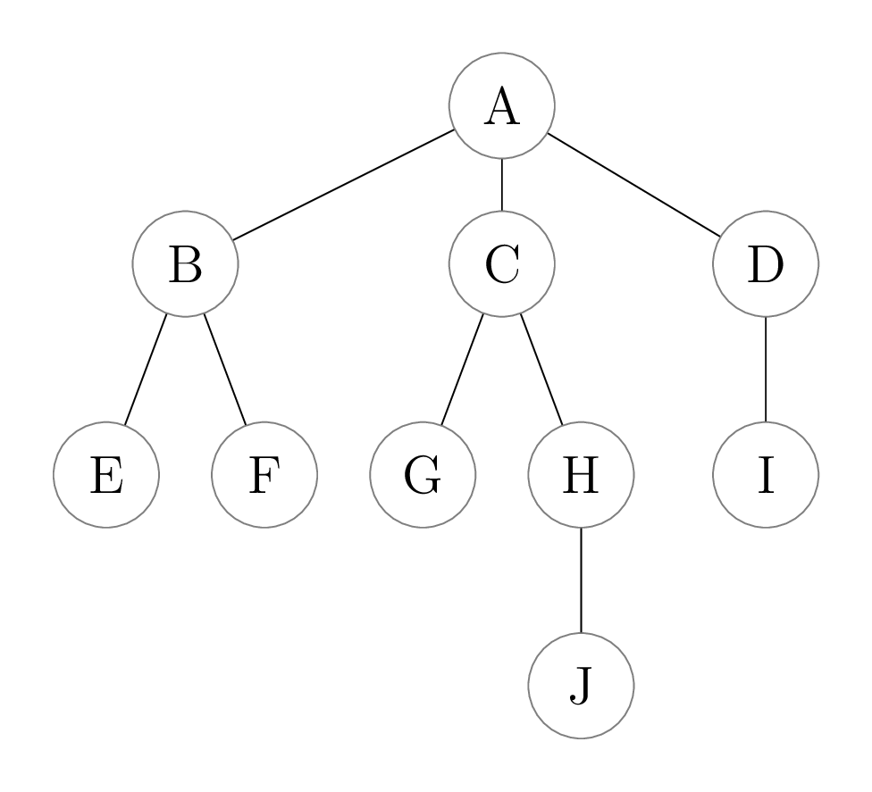
To get around this problem, we need one key observation. Let’s look at an example first. Suppose we have the following tree:
We first identify all recursive calls that are made when we call
__len__ on this tree. Let’s see what happens when we make
our initial call, on the whole tree (rooted at
A). In the bullet points, we identify a tree by naming its
root, e.g. saying “(A)” as shorthand for “the tree rooted at
A”.
- Initial call (A) makes three recursive calls on each of its subtrees
(B), (C), and (D).
- The recursive call on (B) makes two recursive calls on each of its
subtrees, (E) and (F).
- Each of (E) and (F) is a leaf, so no more recursive calls are made from them.
- The recursive call on (C) makes two recursive calls, on (G) and (H).
- The (G) is a leaf, so no more recursive calls happen for that tree.
- The recursive call on (H) makes one more recursive call on (J).
- The (J) is a leaf, so no more recursive calls happen.
- The recursive call on (D) makes more one call, on (I).
- The (I) is a leaf, so no more recursive calls happen.
- The recursive call on (B) makes two recursive calls on each of its
subtrees, (E) and (F).
That’s a lot of writing, but the key takeaway is this: because
__len__’s recursive step always makes a recursive call on
every subtree, in total there is one __len__ call made per
item in the tree. So in our example tree with 10 items, there are 10
calls to __len__ made, including the initial function call
on the whole tree. In other words, the structure of the recursive calls
exactly follows the structure of the tree.
Analyzing the “non-recursive” part of each call
Based on our previous discussion, you might be thinking: so in
general if we have a tree of size \(n\), then \(n\) recursive calls are made, and so the
running time of Tree.__len__ is \(\Theta(n)\). This is on the right track,
but isn’t complete: we can’t just count the number of recursive calls,
since each call might perform other operations as well.
In the case of __len__, the recursive step is the
following:
        else:
            size_so_far = 1
            for subtree in self._subtrees:
                size_so_far += subtree.__len__()
            return size_so_far
In addition to making recursive calls, there are some constant time operations, and a for loop that adds to an accumulator. How do we take into account the number of steps performed by these actions? Essentially what we need to do is count the number of steps performed by a single recursive call, and add those up across all the different recursive calls that are made. This is analogous to computing the cost of a single loop iteration, and then adding the costs up across all loop iterations.
Here is our approach: for the recursive step, we’ll count the number
of steps taken, assuming each recursive call takes constant
time. In effect, we’re counting only the “non-recursive” steps in
the code. So for Tree.__len__, the total number of steps
taken is:
- 1 step for the initial assignment statement
(
size_so_far = 1). - \(k\) steps for the loop, where \(k\) is the number of subtrees in the tree (which determines the number of loop iterations). Note that we’re counting the loop body as just 1 step!
- 1 step for the final return statement.
This gives us a total of \(k + 2\) steps for the non-recursive cost of the else branch. To find the total running time, we need to sum this up across all recursive calls.
So if there are \(n\) recursive calls in total, does this mean the total running time is \(n(k + 2)\)? No! The challenge here is that \(k\), the number of subtrees, changes for each recursive call. In our above example, the full tree (rooted at A) has \(k = 3\), but the tree rooted at B has \(k = 2\), and the tree rooted at E has \(k = 0\). That’s okay—let’s look at what happens when we write these costs for every recursive call in our example tree: We’ve bolded the \(k\) and kept the \(+ 2\) separated so you can see the part that’s changing for each node.
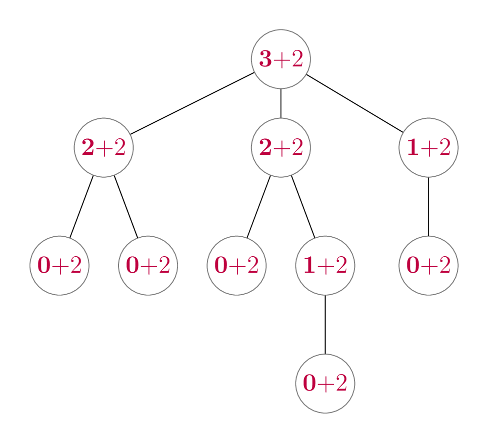
The numbers in this tree represent the total number of steps
taken by our initial call to Tree.__len__, across all the
recursive calls that are made. Let’s add up the example numbers, but in
a slightly smart way: we’ll add up the “\(k\)” and “\(+
2\)” values separately:
\[\begin{align*} & \, \mathbf{3} + 2 \tag{A} \\ +& \, \mathbf{2} + 2 \tag{B} \\ +& \, \mathbf{2} + 2 \tag{C} \\ +& \, \mathbf{1} + 2 \tag{D} \\ +& \, \mathbf{0} + 2 \tag{E} \\ +& \, \mathbf{0} + 2 \tag{F} \\ +& \, \mathbf{0} + 2 \tag{G} \\ +& \, \mathbf{1} + 2 \tag{H} \\ +& \, \mathbf{0} + 2 \tag{I} \\ +& \, \mathbf{0} + 2 \tag{J} \\ \hline =& \, \mathbf{9} + 20 \\ =& \, 29 \end{align*}\]
The second-last line is critical. Let’s break that down:
- The sum of all the subtrees is 9, which is one less than the total number of items. This should make sense, because each non-root item has exactly one parent, it is counted in exactly one subtree.
- The 20 is the constant number of steps (2) multiplied by the number of recursive calls, which is equal to the number of items (10).
Generalize!
Now let’s generalize the above argument to non-empty trees of any size. Let \(n \in \Z^+\), and suppose we have a tree of size \(n\). We know that there will be \(n\) recursive calls made.
- The “constant time” parts will take \(2n\) steps across all \(n\) recursive calls.
- The total number of steps taken by the for loop across all recursive calls is equal to the sum of all of the numbers of children of each node, which is \(n - 1\). Formally proving this statement is beyond the scope of the course. You can do it using a different form of induction which you’ll learn about in CSC236/240.
This gives us a total running time of \(2n + (n - 1) = 3n - 1\), which is \(\Theta(n)\).
Looking back
Because we’ve emphasized the recursive tree method code template so much in the past few sections, it should not be surprising that the above technique really applies to any tree method of the form
class Tree:
    def method(self) -> ...:
        if self.is_empty():
            ...
        else:
            ...
            for subtree in self._subtrees:
                ... subtree.method() ...
            ...
as long as each of the ... is filled in with
constant-time operations. And don’t forget about worst-case running time
either: when we implement Tree.__contains__ using the
pattern, we can use an early return so that the recursive step doesn’t
necessarily recurse on all subtrees. It is possible to show that the
worst-case running time of this method would be \(\Theta(n)\) using the approach described in
this
section.This is a good exercise to practice doing a worst-case
running time analysis!