9.8 Worst-Case Running Time Analysis

In 9.5 Analyzing Algorithm Running Time, we saw how to use asymptotic notation to characterize the rate of growth of the number of “basic operations” as a way of analyzing the running time of an algorithm. This approach allows us to ignore details of the computing environment in which the algorithm is run, and machine- and language-dependent implementations of primitive operations, and instead characterize the relationship between the input size and number of basic operations performed.

However, this focus on just the input size is a little too restrictive. Even though we can define input size differently for each algorithm we analyze, we tend not to stray too far from the “natural” definitions (e.g., length of list). In practice, though, algorithms often depend on the actual value of the input, not just its size. For example, consider the following function, which searches for an even number in a list of integers. This is very similar to how the in operator is implemented for Python lists.

def has_even(numbers: list[int]) -> bool:
    """Return whether numbers contains an even element."""
    for number in numbers:
        if number % 2 == 0:
            return True
    return False

Because this function returns as soon as it finds an even number in the list, its running time is not necessarily proportional to the length of the input list.

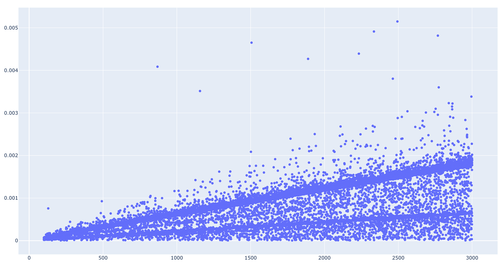
The running time of a function can vary even when the input size is fixed. Or using the notation we learned earlier this chapter, the inputs in \(\cI_{has\_even, 10}\) do not all have the same runtime. The question “what is the running time of has_even on an input of length \(n\)?” does not make sense, as for a given input the runtime depends not just on its length but on which of its elements are even. We illustrate in the following plot, which shows the results of using timeit to measure the running time of has_evens on randomly-chosen lists. While every timing experiment has some inherent uncertainty in the results, the spread of running times cannot be explained by that alone!

Because our asymptotic notation is used to describe the growth rate of functions, we cannot use it to describe the growth of a whole range of values with respect to increasing input sizes. A natural approach to fix this problem is to focus on the maximum of this range, which corresponds to the slowest the algorithm could run for a given input size.

Note that \(WC_{func}\) is a function, not a (constant) number: it returns the maximum possible running time for an input of size \(n\), for every natural number \(n\). And because it is a function, we can use asymptotic notation to describe it, saying things like “the worst-case running time of this function is \(\Theta(n^2)\).”

The goal of a worst-case runtime analysis for func is to find an elementary function \(f\) such that \(WC_{func} \in \Theta(f)\).

However, it takes a bit more work to obtain tight bounds on a worst-case running time than on the runtime functions of the previous section. It is difficult to compute the exact maximum number of basic operations performed by this algorithm for every input size, which requires that we identify an input for each input size, count its maximum number of basic operations, and then prove that every input of this size takes at most this number of operations. Instead, we will generally take a two-pronged approach: proving matching upper and lower bounds on the worst-case running time of our algorithm.

Upper bounds on the worst-case runtime

To get some intuition about what an upper bound on the worst-case running means, suppose we use absolute dominance rather than Big-O. In this case, there’s a very intuitive way to expand the phrase “\(WC_{func}\) is absolutely dominated by \(f\)”:

\[\begin{align*} &\forall n \in \N,~ WC_{func}(n) \leq f(n) \\ \Longleftrightarrow \, &\forall n \in \N,~ \max \big\{ \text{running time of executing $func(x)$} \mid x \in \cI_{func, n} \big\} \leq f(n) \\ \Longleftrightarrow \, &\forall n \in \N,~ \forall x \in \cI_{func, n},~ \text{running time of executing $func(x)$} \leq f(n) \end{align*}\]

The last line comes from the fact that if we know the maximum of a set of numbers is less than some value \(K\), then all numbers in that set must be less than \(K\). Thus an upper bound on the worst-case runtime is equivalent to an upper bound on the runtimes of all inputs.

Now when we apply the definition of Big-O instead of absolute dominance, we get the following translation of \(WC_{func} \in \cO(f)\):

\[ \exists c, n_0 \in \R^+,~ \forall n \in \N,~ n \geq n_0 \Rightarrow \big(\forall x \in \cI_{func, n},~ \text{running time of executing $func(x)$} \leq c \cdot f(n) \big) \]

To approach an analysis of an upper bound on the worst-case, we typically find a function \(g\) such that \(WC_{func}\) is absolutely dominated by \(g\), and then find a simple function \(f\) such that \(g \in \cO(f)\). But how do we find such a \(g\)? And what does it mean to upper bound all runtimes of a given input size? We’ll illustrate the technique in our next example.

Note that we did not prove that has_even(numbers) takes exactly \(n + 1\) basic operations for an arbitrary input numbers (this is false); we only proved an upper bound on the number of operations. And in fact, we don’t even care that much about the exact number: what we ultimately care about is the asymptotic growth rate, which is linear for \(n + 1\). This allowed us to conclude that the worst-case running time of has_even is \(\cO(n)\).

But because we calculated an upper bound rather than an exact number of steps, we can only conclude a Big-O, not Theta bound: we don’t yet know that this upper bound is tight.If this is surprising, note that we could have done the above proof but replaced \(n+1\) by \(5000n + 110\) and it would still have been mathematically valid.

Lower bounds on the worst-case runtime

So how do we prove our upper bound is tight? Since we’ve just shown that \(WC_{has\_even}(n) \in \cO(n)\), we need to prove the corresponding lower bound \(WC_{has\_even}(n) \in \Omega(n)\). But what does it mean to prove a lower bound on the maximum of a set of numbers? Suppose we have a set of numbers \(S\), and say that “the maximum of \(S\) is at least \(50\).” This doesn’t tell us what the maximum of \(S\) actually is, but it does give us one piece of information: there has to be a number in \(S\) which is at least \(50\).

The key insight is that the converse is also true—if I tell you that \(S\) contains the number \(50\), then you can conclude that the maximum of \(S\) is at least \(50\). \[\max(S) \geq 50 \IFF (\exists x \in S,~ x \geq 50)\] Using this idea, we’ll give a formal definition for a lower bound on the worst-case runtime of an algorithm.

Remarkably, the crucial difference between this definition and the one for upper bounds is a change of quantifier: now the input \(x\) is existentially quantified, meaning we get to pick it. Or really, our goal is to find an input family—a set of inputs, one per input size \(n\)—whose runtime is asymptotically larger than our target lower bound.

For example, in has_even we want to prove that the worst-case running time is \(\Omega(n)\) to match the \(\cO(n)\) upper bound, and so we want to find and input family where the number of steps taken is \(\Omega(n)\). Let’s do that now.

Putting it all together

Finally, we can combine our upper and lower bounds on \(WC_{has\_even}\) to obtain a tight asymptotic bound.

To summarize, to obtain a tight bound on the worst-case running time of a function, we need to do two things:

• Use the properties of the code to obtain an asymptotic upper bound on the worst-case running time. We would say something like \(WC_{func} \in \cO(f)\).

• Find a family of inputs whose running time is \(\Omega(f)\). Almost always we find an input family whose running time is \(\Theta(f)\), but strictly speaking only \(\Omega(f)\) is required. This will prove that \(WC_{func} \in \Omega(f)\).

• After showing that \(WC_{func} \in \cO(f)\) and \(WC_{func} \in \Omega(f)\), we can conclude that \(WC_f \in \Theta(f)\).

A note about best-case runtime

In this section, we focused on worst-case runtime, the result of taking the maximum runtime for every input size. It is also possible to define a best-case runtime function by taking the minimum possible runtimes, and obtain tight bounds on the best case through an analysis that is completely analogous to the one we just performed. In practice, however, the best-case runtime of an algorithm is usually not as useful to know—we care far more about knowing just how slow an algorithm is than how fast it can be.

Early returning in Python built-ins

We’ve encountered a few different Python functions and methods whose running time depends on more than just the size of their inputs. We alluded to one at the start of this chapter: the list search operation using the keyword in:

>>> lst = list(range(0, 1000000))
>>> timeit.timeit('0 in lst', number=10, globals=globals())
8.299997716676444e-06
>>> timeit.timeit('-1 in lst', number=10, globals=globals())
0.17990550000104122

In the first timeit expression, 0 appears as the first element of lst, and so is found immediately when the search occurs. In the second, -1 does not appear in lst at all, and so all one-million elements of lst must be checked, resulting in a running-time that is proportional to the length of the list. The worst-case running time of the in operation for lists is \(\Theta(n)\), where \(n\) is the length of the list.

We have also seen two more functions that are implemented using an early return: any and all. Because any searches for a single True in a collection, it stops the first time it finds one. Similarly, because all requires that all elements of a collection be True, it stops the first time it finds a False value.

>>> all_trues = [True] * 1000000
>>> all_falses = [False] * 1000000
>>> timeit.timeit('any(all_trues)', number=10, globals=globals())
8.600000001024455e-06
>>> timeit.timeit('any(all_falses)', number=10, globals=globals())
0.10643419999905745
>>> timeit.timeit('all(all_trues)', number=10, globals=globals())
0.10217570000168053
>>> timeit.timeit('all(all_falses)', number=10, globals=globals())
6.300000677583739e-06

So in the above example:

• any(all_trues) returns True immediately after checking the first list element.
• any(all_falses) returns False only after checking all one-million list elements.
• all(all_trues) returns True only after checking all one-million list elements.
• all(all_falses) returns False immediately after checking the first list element.

So any and all have a worst-case running time of \(\Theta(n)\), where \(n\) is the size of the input collection. But in practice they can be much faster if they encounter the “right” boolean value early on!

any, all, and comprehensions

There is one subtlety that often catches students by surprise when they attempt to call any/all on a comprehension and expect a quick result. Let’s see a simple example:

>>> timeit.timeit('any([x == 0 for x in range(0, 1000000)])', number=10)
0.7032962000012049

That’s a lot slower than we would expect, given that the first element checked is x = 0! The result is similar if we try to use a set comprehension instead of a list comprehension:

>>> timeit.timeit('any({x == 0 for x in range(0, 1000000)})', number=10)
0.6538308000017423

The subtlety here is that in both cases, the full comprehension is evaluated before any is called. As we discussed in [8.5 Analyzing Comprehensions and While Loops], the running time of evaluating a comprehension is proportional to the size of the source collection of the comprehension—in our example, that’s range(0, 1000000), which contains one-million numbers.

But all is not lost! In practice, Python programmers do use any/all with comprehensions, but they do so by writing the comprehension expression in the function call without any surrounding square brackets or curly braces:

>>> any(x == 0 for x in range(0, 1000000))
True

This is called a generator comprehension, and is used to produce a special Python collection data type called a generator. We won’t use generators or generator comprehensions very much at all in this course, but what we want you to know about them here is that unlike set/list comprehensions, generator comprehensions do not evaluate their elements all at once, but instead only when they are needed by the function being called. This means that our above any call achieves the fast running time we initially expected:

>>> timeit.timeit('any(x == 0 for x in range(0, 1000000))', number=10)
4.050000279676169e-05

Now, only the x = 0 value from the generator comprehension gets evaluated; none of the other possible values (x = 1, 2, ..., 999999) are ever checked by the any call!

Don’t assume bounds are tight!

It is likely unsatisfying to hear that upper and lower bounds really are distinct things that must be computed separately. Our intuition here pulls us towards the bounds being “obviously” the same, but this is really a side effect of the examples we have studied so far in this section being rather straightforward. But this won’t always be the case: the study of more complex algorithms and data structures exhibits quite a few situations where obtaining an upper bound on the running time involves a completely different analysis than the lower bound.

Let’s look at one such example that deals with manipulating strings.

def palindrome_prefix(s: str) -> int:
    n = len(s)
    for prefix_length in range(n, 0, -1):  # goes from n down to 1
        # Check whether s[0:prefix_length] is a palindrome
        is_palindrome = all(s[i] == s[prefix_length - 1 - i]
                            for i in range(0, prefix_length))

        # If a palindrome prefix is found, return the current length.
        if is_palindrome:
            return prefix_length