Iterative algorithms are typically quite straightforward to analyse, as long as you can determine precisely how many iterations each loop will run. Recursive code can be trickier, because not only do you need to analyse the running time of the non-recursive part of the code, you must also factor in the cost of each recursive call made.
You’ll learn how to do this formally in CSC236, but for this course we’re going to see a nice visual intuition for analysing simple recursive functions.
Mergesort
Recall the mergesort algorithm:
def mergesort(lst):
    if len(lst) < 2:
        return lst[:]
    else:
        mid = len(lst) // 2 # This is the midpoint of lst
        left_sorted = mergesort(lst[:mid])
        right_sorted = mergesort(lst[mid:])

        return _merge(left_sorted, right_sorted)
Suppose we call mergesort on a list of length n, where n ≥ 2. We first analyze the running time of the code in the branch other than the recursive calls themselves:
- The “divide” step takes linear time, since the list slicing operations
lst[:mid]andlst[mid:]each take roughly n/2 steps to make a copy of the left and right halves of the list, respectively.Note that while this slicing occurs in the same line as a recursive call, the slicing itself is considered non-recursive, since it occurs before making the recursive calls. - The
_mergeoperation also takes linear time, that is, approximately n steps (why?). - The other operations (calling
len(lst), arithmetic, and the act ofreturning) all take constant time, independent of n.
Putting this together, we say that the running time of the non-recursive part of this algorithm is O(n), or linear with respect to the length of the list.
But so far we have ignored the cost of the two recursive calls. Well, since we split the list in half, each new list on which we make a call has length n/2, and each of those merge and slice operations will take approximately n/2 steps, and then these two recursive calls will make four recursive calls, each on a list of length n/4, etc.
We can represent the total cost as a big tree, where at the top level we write the cost of the merge operation for the original recursive call, at the second level are the two recursive calls on lists of size n/2, and so on until we reach the base case (lists of length 1).
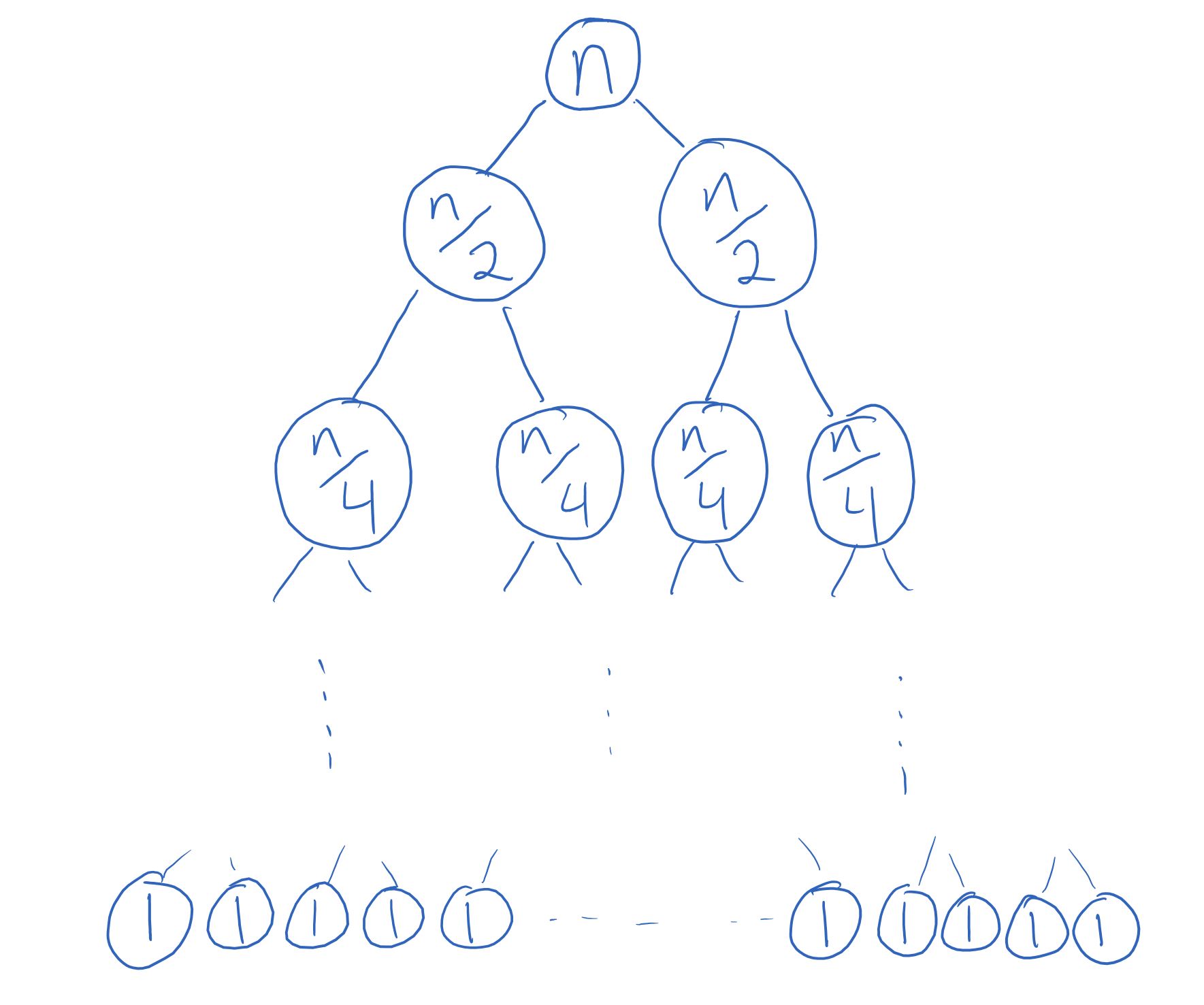
Note that even though it looks like the tree shows the size of the lists at each recursive call, what it’s actually showing is the running time of the non-recursive part of each recursive call, which just happens to be (approximately) equal to the size of the list!
The height of this tree is the recursion depth: the number of recursive calls that are made before the base case is reached. Since for mergesort we start with a list of length n and divide the length by 2 until we reach a list of length 1, the recursion depth of mergesort is the number of times you need to divide n by 2 to get 1. Put another way, it’s the number k such that 2k ≈ n. Remember logarithms? This is precisely the definition: k ≈ log n, and so there are approximately log n levels.Remember that when we omit the base of a logarithm in computer science, we assume the base is 2, not 10.
Finally, notice that at each level, the total cost is n. This makes the total cost of mergesort O(nlog n), which is much better than the quadratic n2 runtime of insertion and selection sort when n gets very large!
You may have noticed that this analysis only depends on the size of the input list, and not the contents of the list; in other words, the same work and recursive calls will be made regardless of the order of the items in the original list. The worst-case and best-case Big-Oh running times for mergesort are the same: O(nlog n).
The Perils of Quicksort
What about quicksort? Is it possible to do the same analysis? Not quite. The key difference is that with mergesort we know that we’re splitting up the list into two equal halves (each of size n/2); this isn’t necessarily the case with quicksort!
Suppose we get lucky, and at each recursive call we choose the pivot to be the median of the list, so that the two partitions both have size (roughly) n/2. Then problem solved, the analysis is the same as mergesort, and we get the nlog n runtime.Something to think about: what do we need to know about _partition for the analysis to be the same? Why is this true?
But what if we’re always extremely unlucky with the choice of pivot: say, we always choose the smallest element? Then the partitions are as uneven as possible, with one having no elements, and the other having size n − 1. We get the following tree: Note that the “1” squares down the tree represent the cost of making the recursive call on an empty list.
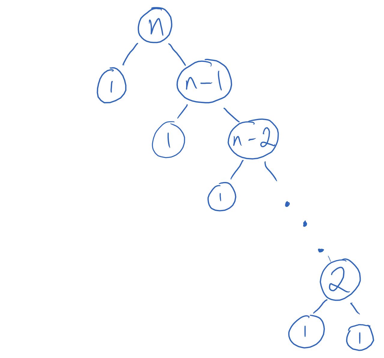
Here, the recursion depth is n (the size decreases by 1 at each recursive call), so adding the cost of each level gives us the expression (n − 1) + [n + (n − 1) + (n − 2) + ... + 1] = (n − 1) + n(n + 1)/2, making the runtime be quadratic.
This means that for quicksort, the choice of pivot is extremely important, because if we repeatedly choose bad pivots, the runtime gets much worse! Its best-case running time is O(nlog n), while its worst-case running time is O(n2).
Quicksort in the “real world”
You might wonder if quicksort is truly used in practice, if its worst-case performance is so much worse than mergesort’s. Keep in mind that we’ve swept a lot of details under the rug by saying that both _merge and _partition take O(n) steps—the Big-Oh expression ignores constant factors, and so 5n and 100n are both treated as O(n) even though they are quite different numerically.
In practice, the non-recursive parts of quicksort can be significantly faster than the non-recursive parts of mergesort. For most inputs, quicksort has “smaller constants” than mergesort, meaning that it takes a fewer number of computer operations, and so performed faster.
In fact, with some more background in probability theory, we can even talk about the performance of quicksort on a random list of length n; it turns out that the average performance is O(nlog n)—with a smaller constant than mergesort’s O(nlog n)—indicating that the actual “bad” inputs for quicksort are quite rare. You will see this proven formally in CSC263/5.