CSC111 Tutorial 5: Binary Search Trees and Recursion Running-Time Analysis

Last week you learned about binary search trees, an application of trees to storing collections of data. In this tutorial, you’ll get more practice working with binary search trees. You’ll also analyze the running time of recursive functions for a variety of data types, which serves as a review of the different recursive data types we have studied over the past few weeks.

Part 1: BinarySearchTree practice

To start, please download tutorial5.py. This file contains the BinarySearchTree class we studied last week.

Your task in this section is to implement the two new methods BinarySearchTree.height and BinarySearchTree.items_in_range. For both of these methods, you’ll need to think carefully about whether you can use the BST property to reduce the number of recursive calls made. Remember our recursive design recipe: write out what the recursive calls on each subtree would return, and think about how to combine these to get the final result.

Notes:

• For BinarySearchTree.height, remember that our definition of height counts the number of items, not the number of edges (parent-to-child connections), on the longest path from the root to a leaf of the tree.
• BinarySearchTree.items_in_range is similar to the BinarySearchTree.items and BinarySearchTree.smaller methods from last week’s prep. The docstring requires you to ensure that the list is returned in the correct order; do not use a built-in list.sort method or function to accomplish this. Instead, you should exploit the fact that a BST is already “sorted”.

Part 2: Recursion Running-Time Analysis

In this part, you’ll get practice analyzing the running time of recursive functions. To start, make sure to review our procedure for doing a recursive running-time analysis:

1. Identify the recursive call structure (drawing a tree diagram). This will follow the structure of the data!
2. Compute the non-recursive running time for each call. This might be the same for each call, or might change for different calls (in which case you’ll need to idenfity a pattern for the running time).
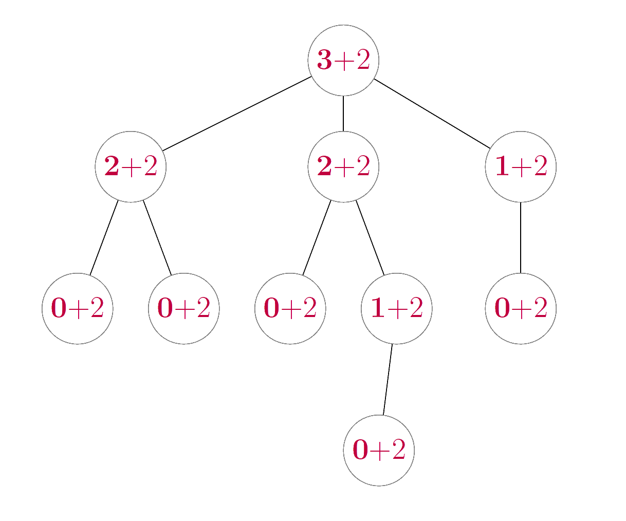
3. Compute the sum of the non-recursive running times across all calls made. We can visualize this first by taking our diagram from (1) and filling in the nodes with the numbers from (2).

Here are two recursion diagrams to help remind you of this process:

In this part of the tutorial, you’ll explore applications of this technique with more complex recursive functions. Pay attention to the class header above each function definition, as we’ve provided examples from all three of RecursiveList, Tree, and BinarySearchTree to help with your review. To simplify your analysis, you can compress all constant-time operations into a single “\(+ 1\) step”. (But note that there may be non-constant time operations as well!!)

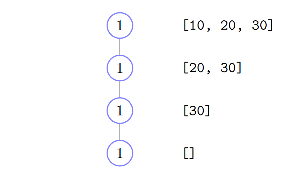
1. Analyze the running time of this function in terms of \(n\), the length of self, and \(m\), the length of numbers.

   class RecursiveList:
       def repeat(self, numbers: list[int]) -> int:
           if self.is_empty():
               return sum(numbers)
           else:
               return self._first + sum(numbers) + self._rest.repeat(numbers)

2. Analyze the running time of this function in terms of \(n\), the length of self, and \(m\), the length of numbers.

   class RecursiveList:
       def sum_both(self, numbers: list[int]) -> int:
           if self.is_empty():
               return sum(numbers)
           else:
               return self._first + self._rest.sum_both(numbers)

3. For this analysis, assume self and numbers have the same length \(n\). Note that list slicing (lst[a:b]) creates a new list, and its running time is equal to the length of the new list (b - a).

   class RecursiveList:
       def sum_products(self, numbers: list[int]) -> int:
           if self.is_empty():
               return 1
           else:
               sum_firsts = self._first * numbers[0]
               numbers_rest = numbers[1:len(numbers)]
   
               return sum_firsts * self._rest.sum_products(numbers_rest)

4. Analyze the running time of this function in terms of \(n\), the size of self, and \(m\), the length of numbers.

   class Tree:
       def sum_all(self, numbers: list[int]) -> int:
           if self.is_empty():
               return 1
           else:
               sum_so_far = self._root * sum(numbers)
               for subtree in self._subtrees:
                   sum_so_far += subtree.sum_all(numbers)
               return sum_so_far

5. Analyze the running time of this function in terms of \(n\), the size of self. For this function you may ignore the running time of recursive calls on empty subtrees (don’t need to draw them in your diagram, or count them in your final sum).

   class BinarySearchTree:
       def sum_all(self) -> int:
           if self.is_empty():
               return 0
           else:
               return self._root + self._left.sum_all() + self._right.sum_all()

6. Analyze the worst-case running time in terms of \(h\), the height (not size!) of self, and \(m\), the size of numbers.

   class BinarySearchTree:
       def sum_left_path(self, numbers: list[int]) -> int:
           if self.is_empty():
               return sum(numbers)
           else:
               return self._root + self._left.sum_left_path(numbers)

Part 3: Rotations

As we discussed in lecture, repeated insertion and deletion operations on a BST can result in a very unbalanced tree, which increases the running time of BST operations. One strategy to resolve this imbalance is to change the structure of the tree itself; we’ll explore one simple version of this for the last part of today’s tutorial.

A rotation is a mutation of a BST that changes the structure of the tree around the root. In a rotation, the root value is “demoted” to a subtree, and a child of the root, called the pivot, is “promoted” to become the new root. There are two kinds of rotations, called left and right rotations, based on which child of the root is selected as the pivot.

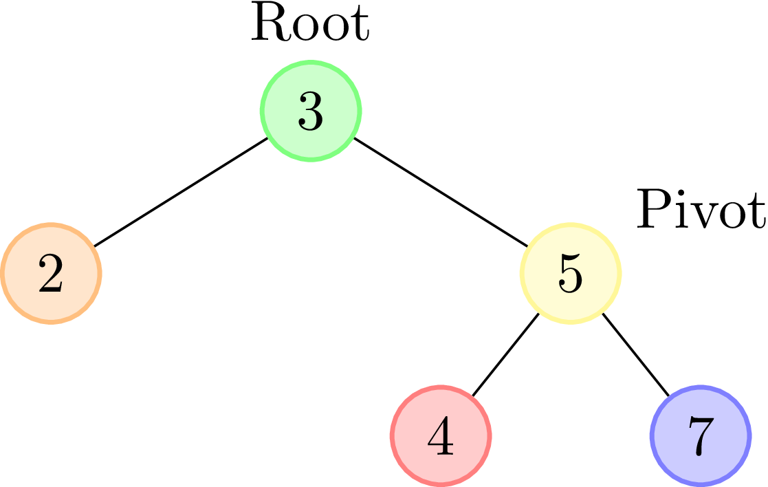
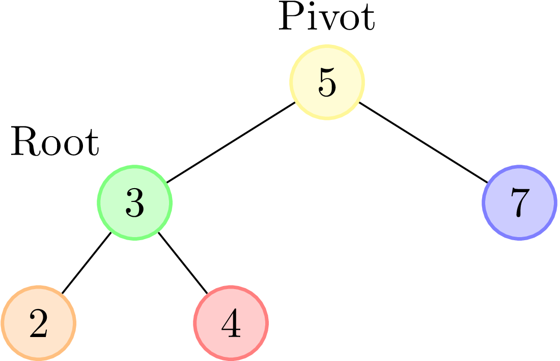
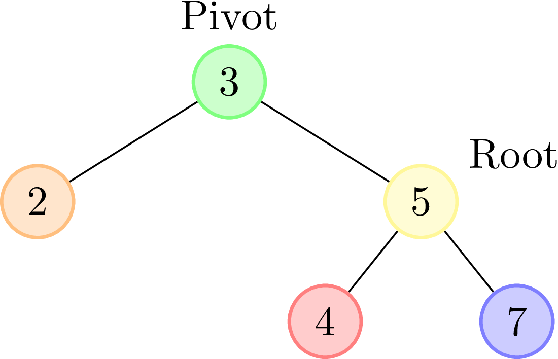
In a left rotation, the right child of the root is the pivot, as in these before and after images:¹

In a right rotation, the left child of the root is the pivot:

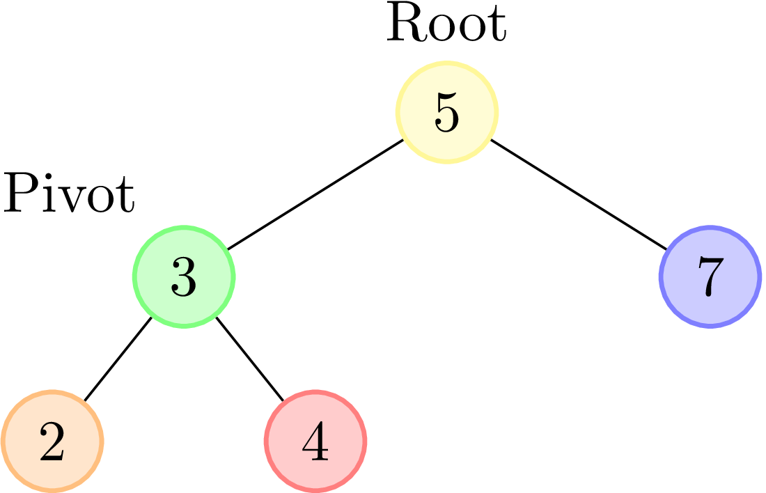
Note: the items 2, 4, and 7 in the above diagrams are drawn as leaves, but really could represent larger trees. Whether or not they have non-empty subtrees doesn’t affect the rotations.

1. Your task is to implement a left and a right rotation as methods of the BinarySearchTree class. Before you start writing any code, draw a few examples of a tree, and practice rotating it to the left, and to the right. Write down the steps involved (i.e., which attributes need to be reassigned) in a left rotation, then write the steps involved in a right rotation.

   Only after you’re confident that you can do these rotations manually should you begin to implement the BinarySearchTree.rotate_left and BinarySearchTree.rotate_right methods in tutorial5.py.

Tips:

1. These rotation methods are not recursive. Instead, they’re an exercise in working carefully with BinarysearchTree attributes.
2. You may create new BinarySearchTrees when implementing these methods.
3. Use parallel assignment to help streamline the tree attribute reassignments in your code.

Looking ahead

With careful use of your rotation methods, it is possible to write BST insertion and deletion methods that ensure that the tree’s height remains logarithmic with respect to its size. The most famous type of binary search tree that uses these rotations is known as the AVL Tree, which you’ll learn all about in CSC263/CSC265.