Exercise 1: In-place partitioning
We’re going to study how to implement an in-place version of
_partition that mutates lst directly, without
creating any new lists. This is the key step to implementing an in-place
version of quicksort.
def _in_place_partition(lst: list) -> None:
    """Mutate lst so that it is partitioned with pivot lst[0].

    Let pivot = lst[0]. The elements of lst are moved around so that lst looks like

        [x1, x2, ... x_m, pivot, y1, y2, ... y_n],

    where each of the x's is <= pivot, and each of the y's is > pivot.

    >>> lst = [10, 3, 20, 5, 16, 30, 7, 100]
    >>> _in_place_partition(lst)  # pivot is 10
    >>> lst[3]  # the 10 is now at index 3
    10
    >>> set(lst[:3]) == {3, 5, 7}
    True
    >>> set(lst[4:]) == {16, 20, 30, 100}
    True
    """
For your reference, there are the diagrams of the example we saw in lecture:
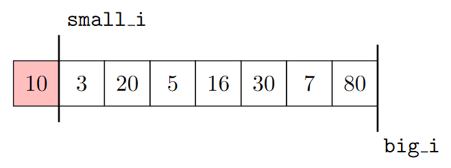
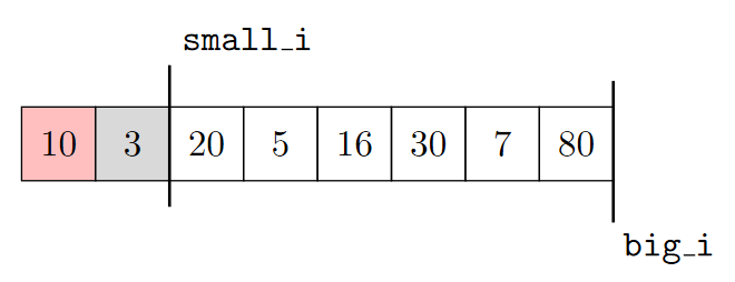
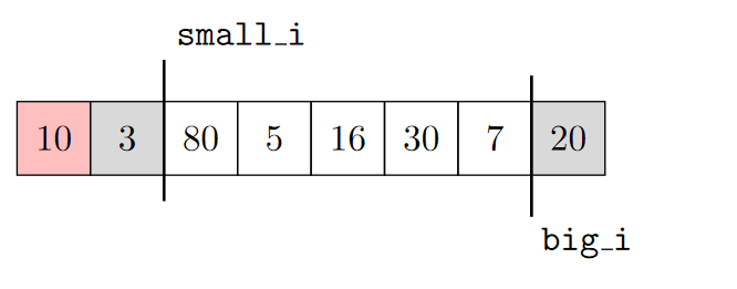
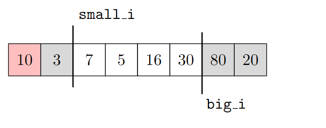
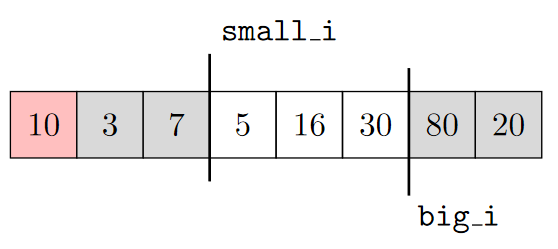
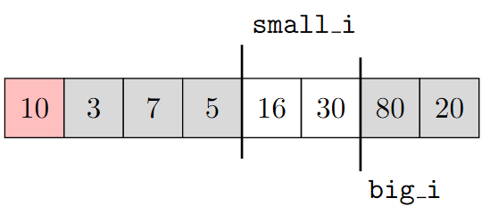
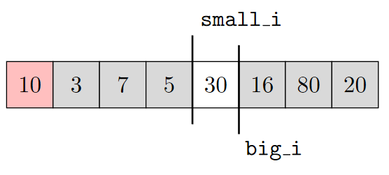
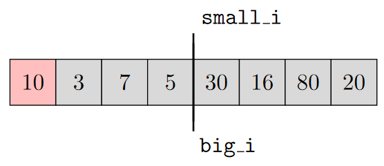
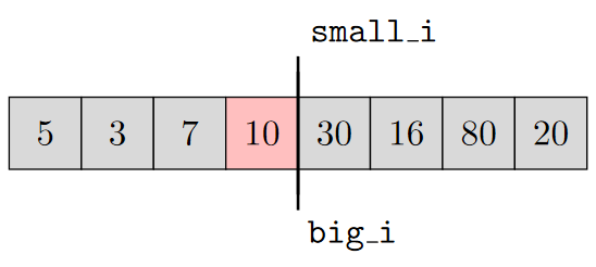
The key idea to implement this function is to divide up
lstinto three parts using indexessmall_iandbig_i:lst[1:small_i]contains the elements that are known to be<= lst[0](the “smaller partition”)lst[big_i:]contains the elements that are known to be> lst[0](the “bigger partition”)lst[small_i:big_i]contains the elements that have not yet been compared to the pivot (the “unsorted section”)
_in_place_partitionuses a loop to go through the elements of the list and compare each one to the pivot, building up either the “smaller” or the “larger partition” and shrinking the “unsorted section.”When we first begin the algorithm, we know that
lst[0]is the pivot, but have not yet compared it against any other list element. What should the initial values ofsmall_iandbig_ibe?We need to check the items one at a time, until every item has been compared against the pivot. What is the relationship between
small_iandbig_iwhen we have finished checking every item?On each loop iteration, the element
lst[small_i]is compared to the pivot.Suppose
lst[small_i]is less than or equal to the pivot, as in the diagram below.![In-place partition, when lst[small_i] is <= the pivot.](images/example1.png)
Which partition should
lst[small_i]belong to? Write the code to updatesmall_ito add this element to the correct the partition.Now suppose
lst[small_i]is greater than the pivot, as in the diagram below.![In-place partition, when lst[small_i] is > the pivot.](images/example2.png)
Which partition should
lst[small_i]belong to? Write the code to swap this element and updatesmall_iorbig_ito add this element to the correct partition.
Next, implement
_in_place_partition. Make sure you’re confident in your answers to the previous questions before writing the main loop!def _in_place_partition(lst: list) -> None: # Initialize variables pivot = lst[0] small_i = big_i = # The main loop # At this point, all elements have been compared. # The final step is to move the pivot into its correct position in the list # (after the "smaller" partition, but before the "bigger" partition).We’re going to need to make this helper a bit more general in order to use it in our a modified quicksort algorithm. If you still have time, complete the following modifications to your implementation of
_in_place_partition.Modify your implementation so that it returns the new index of the pivot in the list (so that when
_in_place_partitionis called in quicksort, we know where the partitions start and end).Modify your implementation so that it takes in two additional parameters
bande, so that the function only partitions the rangelst[b:e]rather than the entire list.
Exercise 2: Running-time analysis for mergesort
Here is our mergesort implementation.
def mergesort(lst: list) -> list:
    if len(lst) < 2:
        return lst.copy()  # Use the list.copy method to return a new list object
    else:
        # Divide the list into two parts, and sort them recursively.
        mid = len(lst) // 2
        left_sorted = mergesort(lst[:mid])
        right_sorted = mergesort(lst[mid:])

        # Merge the two sorted halves. Using a helper here!
        return _merge(left_sorted, right_sorted)
We saw in lecture that the recursive call tree for
mergesort is a binary tree like the following:
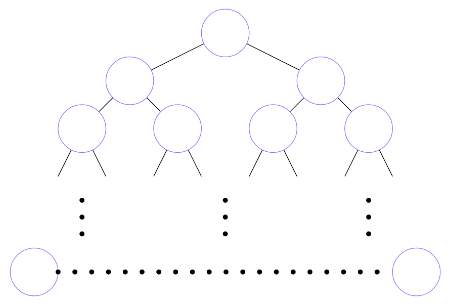
In this exercise, you’ll complete a running-time analysis for mergesort.
Suppose we call
mergesorton a list of length 8. Draw the corresponding recursion diagram, and inside each node write down the non-recursive running time of the call, which we count as equal to the size of the input list for that call.(For example, the root of the tree should contain an “8”, and its two children should be “4”s.)
Compute the total of the numbers in your above diagram. This gives you the total running time for
mergesorton a list of length 8.Now suppose we have a list of length \(n\), where \(n\) is a power of 2. Fill in the recursion diagram below with the corresponding non-recursive running times. The root node should be filled in with \(n\).
Compute the total of the numbers in your above diagram, again assuming \(n\) is a power of 2.
Hint: consider the sum of the numbers in each level of the tree.
Exercise 3: Quicksort running time and uneven partitions
Now consider the quicksort algorithm.
def quicksort(lst: list) -> list:
    if len(lst) < 2:
        return lst.copy()
    else:
        pivot = lst[0]
        smaller, bigger = _partition(lst[1:], pivot)

        smaller_sorted = quicksort(smaller)
        bigger_sorted = quicksort(bigger)

        return smaller_sorted + [pivot] + bigger_sorted
Its recursive step also makes two recursive calls, but unlike mergesort, the input list lengths are not necessarily always the same size.
Suppose we call
quicksort([0, 10, 20, 30, 40]). After the_partitioncall, what aresmallerandbigger?Draw a recursion tree showing the inputs to each recursive call, when we call
quicksort([0, 10, 20, 30, 40]). We’ve started the first two levels for you below. The node containing[]represents a recursive call on an empty list.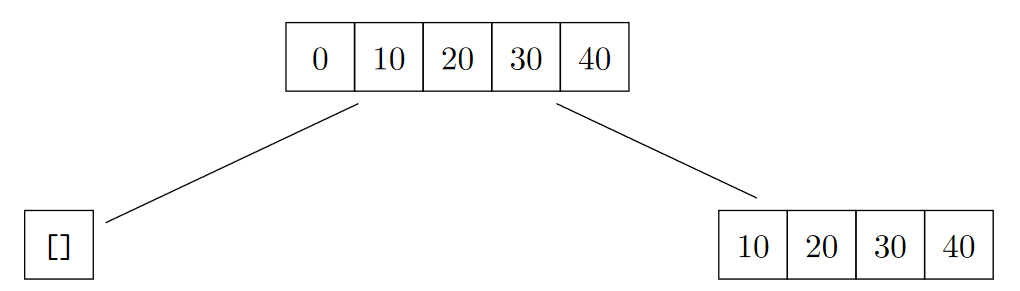
Now redraw the recursion tree, but with the non-recursive running time in each node.
- For an empty list, the non-recursive running time is 1.
- For a non-empty list, the non-recursive running time is the length of the list.
Add up all of the numbers in the above diagram.
Generalize the above calculation for a call to quicksort with a list of length \(n\), when the chosen pivot is always the smallest element in the list.
Additional exercises
To practice the in-place partition algorithms code we covered today, try implementing the following variations.
- Implement
_in_place_partition, but choosing the last element list (lst[-1]) as the pivot instead. - Implement
_in_place_partition_indexed, but choosing the last element of the range (lst[e - 1]) as the pivot instead.
- Implement
Here is the implementation of the helper function
_partitionused by quicksort.def _partition(lst: list, pivot: Any) -> tuple[list, list]: smaller = [] bigger = [] for item in lst: if item <= pivot: smaller.append(item) else: bigger.append(item) return smaller, biggerAnalyze the running time of
_partitionin terms of \(n\), the length of its input list.How would your analysis change if each item were inserted at the front of the relevant list , for example:
smaller.insert(0, item)?
Analyze the running time of your
_in_place_partitionimplementation.In lecture, we saw that our implementation of quicksort (always choosing the first element to be the pivot) has a \(\Theta(n^2)\) running time when given an already-sorted list \([0, 1, \dots, n-1]\). This is because one of the partitions is always an empty list, at every recursive call.
- Find another list that always results in the most unequal partitions (i.e., one of the partitions is always an empty list at every recursive call) with our implementation of quicksort.
- (harder) For a given \(n \in \N^+\) where \(n \geq 2\), find a formula for the number of lists of length \(n\) that result in the most unequal partitions with our implementation of quicksort. Note: this number is \(> 2\).