18.6 Quicksort

In the previous section, we learned about our first divide-and-conquer recursive sorting algorithm, merge sort. Now, we’re going to learn about the second famous such algorithm, which is known as quicksort.

Here’s some intuition for the quicksort approach: suppose we’re sorting a group of people alphabetically by their surname. We do this by first dividing up the people into two groups: those whose surname starts with A-L, and those whose surnames start with M-Z. This can be seen as an “approximate sort”: even though each smaller group is not sorted, we do know that everyone in the A-L group should come before everyone in the M-Z group. Then after sorting each group separately, we’re done: we can simply take the two groups and then concatenate them to obtain a fully sorted list.

The quicksort implementation

Now let’s see how to turn this idea into a more formal algorithm. We’ll follow the structure of a divide-and-conquer approach.

1. First, we pick one element from the input list, which we call the pivot. The implementation we’ll show below always chooses the first element in the list to be the pivot. This has some significant drawbacks, which we’ll discuss in the next section. Then, we split up the list into two parts: the elements less than or equal to the pivot, and those greater than the pivot. This is traditionally called the partitioning step.
2. Next, we sort each part recursively.
3. Finally, we concatenate the two sorted parts, putting the pivot in between them.

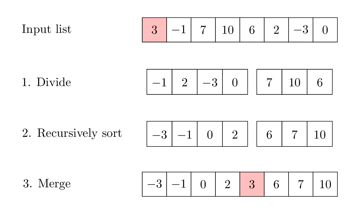
For example, here is how these steps would work for the following list, where we choose the first item in the list as the pivot.

Here is our implementation of a non-mutating version of quicksort. Notice that this has a very similar structure as our mergesort implementation, except now the “divide” step is the hard part that’s pulled out into a helper, while the “combine” step is simple, using just list concatenation.

def quicksort(lst: list) -> list:
    """Return a sorted list with the same elements as lst.

    This is a *non-mutating* version of quicksort; it does not mutate the
    input list.
    """
    if len(lst) < 2:
        return lst.copy()
    else:
        # Divide the list into two parts by picking a pivot and then partitioning the list.
        # In this implementation, we're choosing the first element as the pivot, but
        # we could have made lots of other choices here (e.g., last, random).
        pivot = lst[0]
        smaller, bigger = _partition(lst[1:], pivot)

        # Sort each part recursively
        smaller_sorted = quicksort(smaller)
        bigger_sorted = quicksort(bigger)

        # Combine the two sorted parts. No need for a helper here!
        return smaller_sorted + [pivot] + bigger_sorted

It turns out that implementing the _partition helper is simpler than the _merge helper from mergesort: we can do it just using one loop through the list.

def _partition(lst: list, pivot: Any) -> tuple[list, list]:
    """Return a partition of lst with the chosen pivot.

    Return two lists, where the first contains the items in lst
    that are <= pivot, and the second contains the items in lst that are > pivot.
    """
    smaller = []
    bigger = []

    for item in lst:
        if item <= pivot:
            smaller.append(item)
        else:
            bigger.append(item)

    return (smaller, bigger)

And that’s quicksort! Or at least the non-mutating version. It turns out that we can implement an in-place version of quicksort without too much difficulty (unlike mergesort), and this is something we’ll explore as an exercise in lecture.

Mergesort vs. quicksort

Since we’ve now learned about both mergesort and quicksort, we can compare and contrast these two algorithms, just like we did for selection sort and insertion sort earlier in this chapter.

Both mergesort and quicksort are recursive sorting algorithms based on the divide-and-conquer paradigm. Where they differ, however, is in where they do their “hard work”.

• For mergesort, the “divide” step is simple, since the input list is just split in half. The “combine” step is the hard part, where we use a clever _merge helper to merge the two sorted lists together.
• For quicksort, the “divide” step is the complex one, where the input list is partitioned into two parts based on comparing the items to a chosen pivot value. But once that’s done, the “combine” step is simple: we can just concatenate the results.

So both mergesort and quicksort seem to have one “easy” part and one “hard” part in the divide-and-conquer approach. To complete our comparison of these two algorithms, we’ll need to analyse their running times.After all, we still don’t know why the algorithm is called quicksort. To be continued in the next section!