18.5 Mergesort

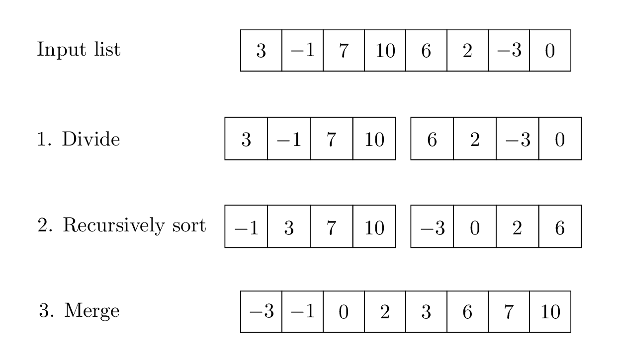
The first divide-and-conquer sorting algorithm we’ll study is called mergesort. This algorithm works as follows:

1. Given an input list to sort, divide the input into the left half and right half.
2. Recursively sort each half.
3. Merge each sorted half together.

As you might expect from this description, in mergesort the “easy” part is dividing the input into halves, and the “hard” part is merging each sorted half into one final sorted list.

For the rest of this section, we’ll discuss how to implement the mergesort algorithm. After we’ve covered both this algorithm and quicksort, we’ll wrap up by discussing running time of these two algorithms.

Implementing mergesort

Here is the specification for our mergesort Python function. Note that we’ll use a non-mutating version, which is a little simpler to work with than the mutating version of mergesort.

def mergesort(lst: list) -> list:
    """Return a new sorted list with the same elements as lst.

    This is a *non-mutating* version of mergesort; it does not mutate the
    input list.
    """

Because our implementation is recursive, we’ll need a base case. Our initial divide-and-conquer description didn’t have a base case, but we can determine an appropriate one by asking, “When can we not divide the list any further?” This occurs when the list has fewer than two elements.

def mergesort(lst: list) -> list:
    """..."""
    if len(lst) < 2:
        return lst.copy()  # Use the list.copy method to return a new list object
    else:
        ...

Now for the recursive step. We need to divide the list into two halves, recursively sort each half, and then merge the sorted halves back together. The first two steps are pretty straightforward:

def mergesort(lst: list) -> list:
    """..."""
    if len(lst) < 2:
        return lst.copy()  # Use the list.copy method to return a new list object
    else:
        # Divide the list into two parts, and sort them recursively.
        mid = len(lst) // 2
        left_sorted = mergesort(lst[:mid])
        right_sorted = mergesort(lst[mid:])

        ...

But how do we merge the two sorted halves? That’s the most complex part of mergesort, and where this sorting algorithm gets its name.

The merge operation

As usual, we’ll separate out the main work into a helper function:

def _merge(lst1: list, lst2: list) -> list:
    """Return a sorted list with the elements in lst1 and lst2.

    Preconditions:
        - is_sorted(lst1)
        - is_sorted(lst2)
    """

How do we implement this function? Intuitively, we can use a similar idea as selection sort: build up a sorted list one element at a time, by repeatedly removing the next smallest element from lst1 or lst2. If the two lists were unsorted, then at each iteration we’d need to iterate through both lists to find their minimum element. But because both lists are sorted, we can determine what that minimum element is very efficiently: simply compare lst1[0] and lst2[0]!

For example, suppose we have the lists lst1 = [-1, 3, 7, 10] and lst2 = [-3, 0, 2, 6]. We can directly compare lst1[0] (which is -1) and lst2[0] (which is -3) to find the smallest element across the two lists, without looking at the other elements in the lists. Here is a table that traces how our merge algorithm will work to build up a sorted list: Compare this to the table in 18.2 Selection Sort.

In each row of the table, the sorted list is built up by one element, until we’ve exhausted one of the lists. After this happens, we don’t need any more comparisons: we can simply concatenate the sorted list with the unmerged items from the remaining list, as the latter will all be >= the former. So our final result is [-3, -1, 0, 2, 3, 6] + [7, 10], yielding the merged sorted list.

Our _merge implementation follows this idea, and is a kind of mixture of the non-in-place and in-place versions of selection sort. We have a new list accumulator to store the sorted list, but also use index variables to act as the boundary between the merged and unmerged items in lst1 and lst2.

def _merge(lst1: list, lst2: list) -> list:
    """Return a sorted list with the elements in lst1 and lst2.

    Preconditions:
        - is_sorted(lst1)
        - is_sorted(lst2)

    >>> _merge([-1, 3, 7, 10], [-3, 0, 2, 6])
    [-3, -1, 0, 2, 3, 6, 7, 10]
    """
    i1, i2 = 0, 0
    sorted_so_far = []

    while i1 < len(lst1) and i2 < len(lst2):
        # Loop invariant:
        # sorted_so_far is a merged version of lst1[:i1] and lst2[:i2]
        assert sorted_so_far == sorted(lst1[:i1] + lst2[:i2])

        if lst1[i1] <= lst2[i2]:
            sorted_so_far.append(lst1[i1])
            i1 += 1
        else:
            sorted_so_far.append(lst2[i2])
            i2 += 1

    # When the loop is over, either i1 == len(lst1) or i2 == len(lst2)
    assert i1 == len(lst1) or i2 == len(lst2)

    # In either case, the remaining unmerged elements can be concatenated to sorted_so_far.
    if i1 == len(lst1):
        return sorted_so_far + lst2[i2:]
    else:
        return sorted_so_far + lst1[i1:]

And finally, here is our completed implementation of mergesort, making use of this _merge helper.

def mergesort(lst: list) -> list:
    """..."""
    if len(lst) < 2:
        return lst.copy()  # Use the list.copy method to return a new list object
    else:
        # Divide the list into two parts, and sort them recursively.
        mid = len(lst) // 2
        left_sorted = mergesort(lst[:mid])
        right_sorted = mergesort(lst[mid:])

        # Merge the two sorted halves. Using a helper here!
        return _merge(left_sorted, right_sorted)

What about an in-place version?

You might wonder about how we can modify our above implementation to create an in-place version of mergesort. Unsurprisingly, the challenging part of such approaches is implementing the _merge step without using an additional list to keep track of the merged elements as the loop progresses. While such in-place _merge—and mergesort—implementations do exist, they’re quite complex, and beyond the scope of this course. For a bit of further reading, check out this Wikipedia section.