18.3 Insertion Sort

In the previous section, we learned about our first sorting algorithm, selection sort. In-place selection sort worked by building up a sorted section of its input list one element at a time. The next sorting algorithm we’ll look at has the same structure, but uses a different approach for how it builds up its sorted section.

Insertion sort idea

The sorting algorithm we’ll study in this section is insertion sort. The in-place version of this algorithm again uses a loop, with a loop variable i to keep track of the boundary between the sorted and unsorted parts of the input list lst.

At loop iteration i, the sorted part is lst[:i]. Unlike selection sort, insertion sort doesn’t choose the smallest unsorted element to add to the sorted part. Instead, it always takes the next item in the list, lst[i], and inserts it into the sorted part by moving it into the correct location to keep this part sorted.

Here’s an example of running in-place insertion sort on the list [3, 0, 1, 8, 7].

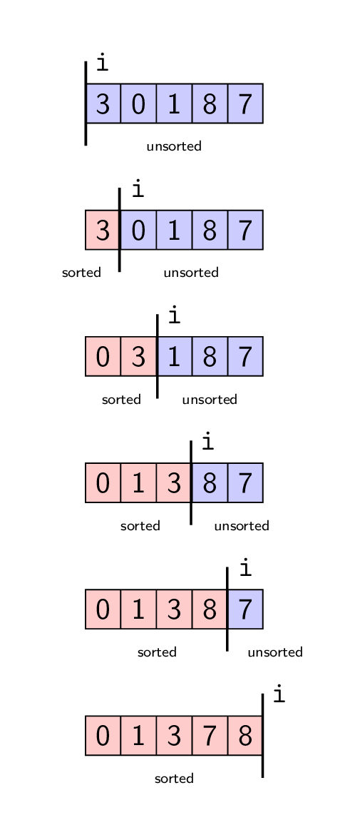
In this example. i starts at 0.

• At iteration i = 0, lst[0] is 3, and since every sublist of length 1 is sorted, we do not need to reposition any items. After this iteration, lst[:1] is sorted.
• At iteration i = 1, lst[1] is 0 and the sorted part is [3]. We need to swap 0 and 3 to make lst[:2] sorted.
• At iteration i = 2, lst[2] is 1 and the sorted part is [0, 3]. We need to swap 1 and 3 to make lst[:3] sorted.
• At iteration i = 3, lst[3] is 8 and the sorted part is [0, 1, 3]. We don’t need to make any swaps (since 8 > 3), and the sorted part is now lst[:4].
• Finally, at iteration i = 4, lst[4] is 7. We need to swap 8 and 7 to make lst[:5] sorted. After this iteration is over, the entire list is sorted!

Loop structure and invariant

Insertion sort has a similar loop structure to selection sort, and shares the key “sorted/unsorted parts” loop invariant as well. Here’s the start of our algorithm:

def insertion_sort(lst: list) -> None:
    """Sort the given list using the insertion sort algorithm.

    Note that this is a *mutating* function.
    """
    for i in range(0, len(lst)):
        assert is_sorted(lst[:i])

        ...


def is_sorted(lst: list) -> bool:
    """Return whether this list is sorted."""
    # Implementation omitted

Note that unlike selection sort, we don’t have a second loop invariant saying that lst[:i] contains the i smallest numbers in the list. Insertion sort doesn’t choose the next smallest number at each loop iteration. Instead, it always takes the next number in the list (lst[i]) and inserts that into the sorted part.

Implementing the loop

To complete our insertion sort implementation, we’ll use a helper function _insert that actually performs the insertion we described above. Since this is a bit more complicated than our helper function for selection sort, we’ll break it down a bit more. Here’s the specification for this function:

def _insert(lst: list, i: int) -> None:
    """Move lst[i] so that lst[:i + 1] is sorted.

    Preconditions:
        - 0 <= i < len(lst)
        - is_sorted(lst[:i])

    >>> lst = [7, 3, 5, 2]
    >>> _insert(lst, 1)
    >>> lst  # lst[:2] is not sorted
    [3, 7, 5, 2]
    """

There are many ways of implementing this helper function. One of the most efficient is to work backwards, repeatedly swapping the item with the one before it until we reach an item that’s <= the item being inserted, or we’ve reached the front of the list.

We’ll show two implementations of this function, one using an early return and one using a compound loop condition. If this sounds familiar, it’s because we showed both of these approaches all the way back in 13.2 Traversing Linked Lists.

# Version 1, using an early return
def _insert(lst: list, i: int) -> None:
    for j in range(i, 0, -1):  # This goes from i down to 1
        if lst[j - 1] <= lst[j]:
            return
        else:
            # Swap lst[j - 1] and lst[j]
            lst[j - 1], lst[j] = lst[j], lst[j - 1]


# Version 2, using a compound loop condition
def _insert(lst: list, i: int) -> None:
    j = i
    while not (j == 0 or lst[j - 1] <= lst[j]):
        # Swap lst[j - 1] and lst[j]
        lst[j - 1], lst[j] = lst[j], lst[j - 1]

        j -= 1

These two implementations do the same thing, but are organized differently. Please make sure that you understand both of them, as it’s good review of the loop techniques we learned about earlier in the course.

With this _insert function complete, we can simply call it inside our main insertion_sort loop:

def insertion_sort(lst: list) -> None:
    """Sort the given list using the insertion sort algorithm.

    Note that this is a *mutating* function.
    """
    for i in range(0, len(lst)):
        assert is_sorted(lst[:i])

        _insert(lst, i)

Running-time analysis for insertion sort

We’ll end off this section analysing the running time of our insertion sort algorithm. To start, we need to analysing the running time of our helper function _insert. We’ll analyse the “early return” implementation, but the same analysis applies to the compound loop condition version as well.

Running-time analysis for _insert. Because of the early return, this function can stop early, and so has a spread of running times. We’ll need to analyse the worst-case running time.

Upper bound: Let \(n \in \N\) and let lst be an arbitrary list of length \(n\). Let \(i \in \N\) and assume \(i < n\). The loop runs at most \(i\) times (for \(j = i, i-1, \dots, 1\)), and each iteration takes constant time (1 step). The total running time of the loop, and therefore the function, is at most \(i\) steps. Therefore the worst-case running time of _insert is \(\cO(i)\).

For a matching lower bound, consider an input list lst where lst[i] is less than all items in lst[:i].For example, a list where lst[j] = 1 for j < i and lst[i] = 0. In this case, the expression lst[j - 1] <= lst[j] will always be False, and so the loop will only stop when j == 0, which takes \(i\) iterations. So for this input, the running time of _insert is \(i\) steps, which is \(\Theta(i)\), matching the upper bound.

So the worst-case running time of _insert is \(\Theta(i)\).

Running-time analysis for insertion_sort. Even though this function doesn’t have any early returns or complex loop conditions, it calls a helper that has a spread of running times, and so insertion_sort also has a spread of running times. We’ll need to analyse its worst-case running time.

Upper bound: Let \(n \in \N\) and let lst be an arbitrary list of length \(n\). The loop iterates \(n\) times, for \(i = 0, 1, \dots, n - 1\). In the loop body, the call to _insert(lst, i) counts as at most \(i\) steps (since its worst-case running time is \(\Theta(i)\)). As usual, we’ll ignore the running time of the assert statement, so the running time of the entire iteration is just \(i\) steps.

This gives us an upper bound on the worst-case running time of \(\sum_{i=0}^{n- 1} i = \frac{n (n - 1)}{2}\), which is \(\cO(n^2)\).

For a matching lower bound, let \(n \in \N\) and let lst be the list \([n - 1, n-2, \dots, 1, 0]\). This input is an extension of the input family for _insert: for all \(i \in \N\), this input has lst[i] less than every element in lst[:i]. As we described above, this causes each call to _insert to take \(i\) steps.

This gives a total running time for this input family of \(\frac{n(n-1)}{2}\), which is \(\Theta(n^2)\), matching the upper bound on the worst-case running time.

Therefore, we can conclude that the worst-case running time of insertion_sort is \(\Theta(n^2)\).

Selection sort vs. insertion sort

Now that we’ve covered both selection sort and insertion sort, let’s take a moment to compare these two algorithms.

Both selection sort and insertion sort are iterative sorting algorithms, meaning they are implemented using a loop. Moreover, both of these algorithms use the same strategy of building up a sorted sublist within their input list, with each loop iteration increasing the size of the sorted part by one.

You can think of the action inside each loop iteration as being divided into two phases: selecting which remaining item to add to the sorted part, and then adding that item to the sorted part. Where these two algorithms differ is in which of these two steps they emphasize. In selection sort, the hard work is done in picking which item to insert next (the smallest one remaining), and the easy part is adding it to the sorted sublist. In insertion sort, the easy part is picking which item to insert (simply the one at index i), and the hard work is inserting that item into the correct spot in the sorted sublist to ensure the resulting sublist is still sorted.

Presented this way, it seems like selection sort and insertion sort are “balanced”: each algorithm has one easy and one hard part in the loop body. But this is where our experience in algorithm analysis allows us to go deeper. Though selection sort and insertion sort both have a worst-case running time of \(\Theta(n^2)\), their running time behaviour is actually very different. Selection sort always takes \(\Theta(n^2)\) steps, regardless of what input it has been given. But insertion sort has a spread of running times, and in particular can be much faster than \(\Theta(n^2)\) on many kinds of inputs, such as lists that are already sorted. To see why, consider what happens with the _insert helper when given a list where lst[i] is >= all items in lst[:i].

So even though these algorithms are very similar both conceptually and in terms of their implementation structure, insertion sort is preferable because of its potential to be more efficient on many different input lists!

References

• CSC108 videos: Insertion Sort (Part 1, Part 2)