16.2 Variables and the Variable Environment

In the last section, we began our study of representing code in a recursive data structure called an abstract syntax tree. We introduced three Python data types: Expr, an abstract class representing an arbitrary type of expression, and its two subclasses Num (representing numeric literals) and BinOp (representing arithmetic operations like + and *). In this section, we’re going to extend what we’ve learned to introduce one new fundamental element of Python programs: variables.

Variables and the Name class

Consider the following Python expression: x + 5.5. This is clearly an arithmetic expression, but its left operand, x, is neither a numeric literal nor a nested arithmetic expression. It is a variable, and so requires a new Expr subclass, which we’ll call Name:

class Name(Expr):
    """A variable expression.

    Instance Attributes:
        - id: The variable name.
    """
    id: str

    def __init__(self, id_: str) -> None:
        """Initialize a new variable expression."""
        self.id = id_

With this class in hand, here is how we can represent the expression x + 5.5:

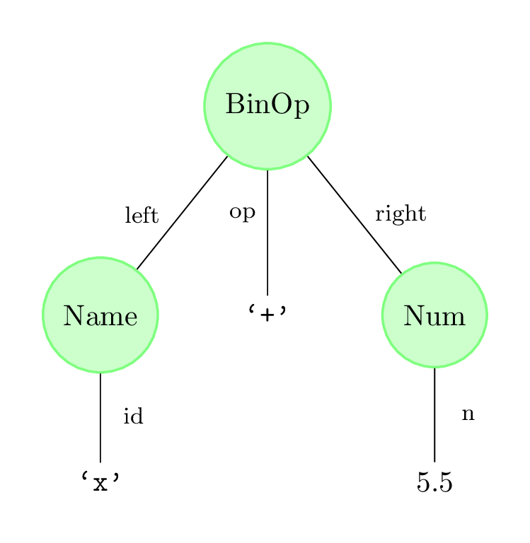
# x + 5.5
BinOp(Name('x'), '+', Num(5.5))

But we shouldn’t just be satisfied with representing this expression—how do we evaluate it?

Evaluating variables by dictionary lookup

Let’s draw inspiration from the Python interpreter. Suppose we type the following into the Python console:

>>> x + 5.5

How does the Python interpreter compute the value of this expression? You might be thinking one of two things:

• x hasn’t been defined yet, so we’d get a NameError!
• Or, it depends on what value x was assigned to earlier in the console.

Both of these thoughts rely on the same underlying behaviour when evaluating variables: the Python interpreter keeps track of what values variables have been assigned to, and then looks up a variable’s current value to evaluate it. Abstractly, this requires a mapping between variable names and values, and so it is perhaps unsurprising that the Python interpreter uses a dict to keep track of this data. The real story is more complex. Python has two built-in functions, globals and locals, and each return separate dictionaries. The former returns the “global variable” dictionary, containing variables that have been defined in the console or at the top-level of the current Python module. The latter returns the “local variable” dictionary, which contains the variables in the local scope wherever it is called (most commonly, inside the body of a function). We call this dictionary the variable environment, and call each key-value pair in the environment a binding between a variable and its current value.

We’ll adapt this idea to modify our abstract syntax tree implementation. This is a fairly large change: we need to modify our Expr.evaluate method header so that it takes an additional argument, env, which contains all of the current variable bindings that can be used when evaluating the expression. Here is how we could update all three of Expr, Num, and BinOp to use this new method form:

class Expr:
    def evaluate(self, env: dict[str, Any]) -> Any:
        """Evaluate this statement with the given environment.

        This should have the same effect as evaluating the statement by the
        real Python interpreter.
        """
        raise NotImplementedError


class Num(Expr):
    def evaluate(self, env: dict[str, Any]) -> Any:
        """..."""
        return self.n  # Simply return the value itself!

class BinOp(Expr):
    def evaluate(self, env: dict[str, Any]) -> Any:
        """..."""
        left_val = self.left.evaluate(env)
        right_val = self.right.evaluate(env)

        if self.op == '+':
            return left_val + right_val
        elif self.op == '*':
            return left_val * right_val
        else:
            raise ValueError(f'Invalid operator {self.op}')

Nothing has changed much: we’ve added the new parameter env, and are passing it into the recursive calls in BinOp.evaluate). But now with this new parameter, we can implement Name.evaluate quite easily.

class Name:
    def evaluate(self, env: dict[str, Any]) -> Any:
        """Return the *value* of this expression.

        The returned value should the result of how this expression would be
        evaluated by the Python interpreter.

        The name should be looked up in the `env` argument to this method.
        Raise a NameError if the name is not found.
        """
        if self.id in env:
            return env[self.id]
        else:
            raise NameError(f"name '{self.id}' is not defined")

Here are two examples of using this method:

>>> expr = Name('x')
>>> expr.evaluate({'x': 10})
10
>>> binop = BinOp(expr, '+', Num(5.5))
>>> binop.evaluate({'x': 100})
105.5

This seems a bit too easy, and you might be wondering: just where do these environments come from? Our two examples used arbitrarily-chosen numbers for x, but we certainly don’t expect (or want) the Python interpreter to generate random variable bindings. To understand how these environments are defined, we’ll need to broaden our implementation of abstract syntax trees to introduce different kinds of statements, such as the assignment statements that determine the value of the current environment. Stay tuned for this in the next section!