To wrap up our study of tree-based data structures in this course, we’re going to look at one particularly rich application of trees: representing programs. Picture a typical Python program you’ve written: a few classes, more than a few functions, and dozens or even hundreds of lines of code. As humans, we read and write code as text, and we take for granted the fact that we can ask the computer to run our code to accomplish pretty amazing things.
But what actually happens when we “run” a program? Another program, called the Python interpreter, is responsible for taking our file and running it. But as you’ve experienced first-hand by now, writing programs that work directly with strings is hard; reading sequences of characters and extracting meaning from them requires a lot of fussing with small details. There’s a fundamental problem with working directly with text: strings are a linear structure (a sequence of characters), but programs are much more complex, and in fact have a naturally recursive structure. Think about all of the different types of Python code we’ve learned so far: arithmetic expressions, lists and other collections, if statements and for loops, for example. Each of these types of code have the potential to be arbitrarily nested, and it is this nesting that makes program structure recursive. Of course, we consider it poor style to write any code that has too much nesting, and tools like PythonTA will complain if you do. But deeply nested code is still valid Python code, and can certainly be run by the Python interpreter.
So the first step that the Python interpreter takes when given a Python file to run is to parse the file’s contents and create a new representation of the program code called an Abstract Syntax Tree (AST). This is, in fact, a simplification: given the complex nature of parsing and Python programs, there is usually more than one kind of tree that is created during the execution of the program, representing different “phases” of the process. You’ll learn about this more in a course on programming languages or compilers, like CSC324 and CSC488. The “Tree” part is significant: given the recursive nature of Python programs, it is natural that we’ll use a tree-based data structure to represent them!
In this chapter, we’re going to explore the basics of modelling programs using abstract syntax trees. In this section we’ll start with the fundamental building blocks of a programming language: expressions that can be evaluated.
The Expr class
Recall that an expression is a piece of code which is meant
to be evaluated, returning the value of that
expression. This is in contrast with statements, which
represent some kind of action like variable assignment or
return, or which represent a definition, using
keywords like def and class.
Expressions are the basic building blocks of the language, and are
necessary for computing anything. But because of the immense variety of
expression types in Python, we cannot use just one single class to
represent all types of expressions. Instead, we’ll use different classes
to represent each kind of expression—but use inheritance to ensure that
they all follow the same fundamental interface.
To begin, here is an abstract class that establishes a common shared interface for all expression types.
class Expr:
    """An abstract class representing a Python expression.
    """
    def evaluate(self) -> Any:
        """Return the *value* of this expression.

        The returned value should be the result of how this expression would be
        evaluated by the Python interpreter.
        """
        raise NotImplementedError
Notice that we haven’t specified any attributes for this class. Every type of expression will use a different set of attributes to represent the expression. Let’s make this concrete by looking at two expression types.
Num: numeric literals
The simplest type of Python expression is a literal like
3 or 'hello'. We’ll start just by representing
numeric literals (ints and floats). As you
might expect, this is a pretty simple class, with just a single
attribute representing the value of the literal.
class Num(Expr):
    """A numeric literal.

    Instance Attributes:
        - n: the value of the literal
    """
    n: int | float

    def __init__(self, number: int | float) -> None:
        """Initialize a new numeric literal."""
        self.n = number

    def evaluate(self) -> Any:
        """Return the *value* of this expression.

        The returned value should be the result of how this expression would be
        evaluated by the Python interpreter.

        >>> expr = Num(10.5)
        >>> expr.evaluate()
        10.5
        """
        return self.n  # Simply return the value itself!
You can think of literals as being the base cases, or leaves, of an abstract syntax tree. Next, we’ll look at one way of combining these literals in larger expressions.
BinOp: arithmetic
operations
The obvious way to combine numbers in code is through the standard
arithmetic operations. In Python, an arithmetic operation is an
expression that consists of three parts: a left and right subexpression
(the two operands of the expression), and the operator itself.
We’ll represent this with the following
class: For simplicity, we restrict the possible operations to
only + and * for this example.
class BinOp(Expr):
    """An arithmetic binary operation.

    Instance Attributes:
        - left: the left operand
        - op: the name of the operator
        - right: the right operand

    Representation Invariants:
        - self.op in {'+', '*'}
    """
    left: Expr
    op: str
    right: Expr

    def __init__(self, left: Expr, op: str, right: Expr) -> None:
        """Initialize a new binary operation expression.

        Preconditions:
            - op in {'+', '*'}
        """
        self.left = left
        self.op = op
        self.right = right
Note that the BinOp class is basically a binary tree!
Its “root” value is the operator name (stored in the attribute
op), while its left and right “subtrees” represent the two
operand subexpressions.
For example, we could represent the simple arithmetic expression
3 + 5.5 in the following way:
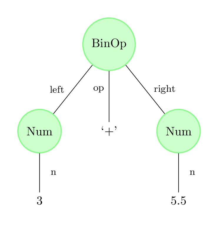
BinOp(Num(3), '+', Num(5.5))But the truly powerful thing about our BinOp data type
is that its left and right attributes aren’t
Nums, they’re Exprs. This is what makes this
data type recursive, and allows it to represent nested arithmetic
operations:
# ((3 + 5.5) * (0.5 + (15.2 * -13.3)))
BinOp(
    BinOp(Num(3), '+', Num(5.5)),
    '*',
    BinOp(
        Num(0.5),
        '+',
        BinOp(Num(15.2), '*', Num(-13.3))))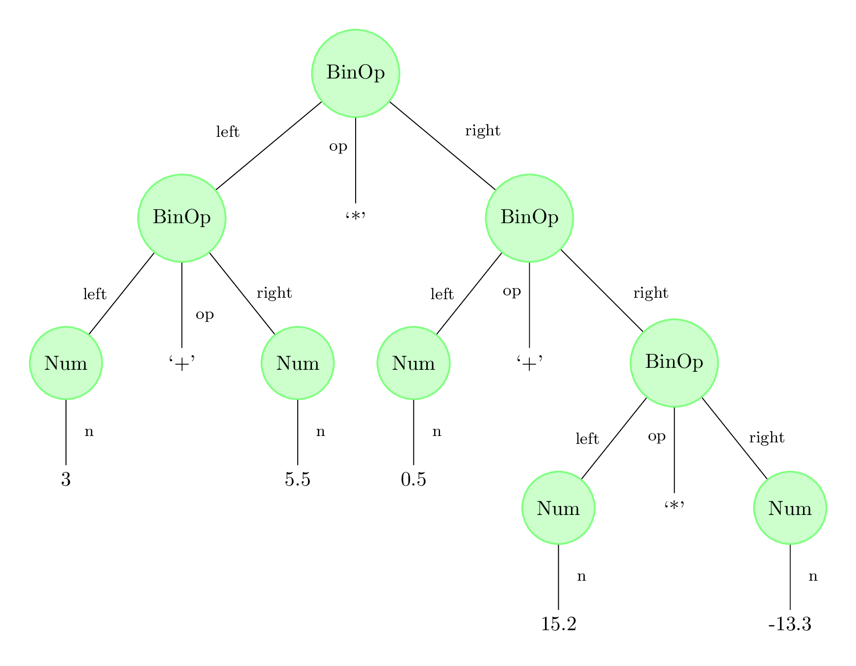
Now, it might seem like this representation is more complicated, and
certainly more verbose. But we must be aware of our own human biases:
because we’re used to reading expressions like
((3 + 5.5) * (0.5 + (15.2 * -13.3))), we take it for
granted that we can quickly parse this text in our heads to
understand its meaning. A computer program like the Python interpreter,
on the other hand, can’t do anything “in its head”: a programmer needs
to have written code for every action it can take! And this is where the
tree-like structure of BinOp really shines. To
evaluate a binary operation, we first evaluate its left and
right operands, and then combine them using the specified arithmetic
operator.
class BinOp:
    def evaluate(self) -> Any:
        """Return the *value* of this expression.

        The returned value should be the result of how this expression would be
        evaluated by the Python interpreter.

        >>> expr = BinOp(Num(10.5), '+', Num(30))
        >>> expr.evaluate()
        40.5
        """
        left_val = self.left.evaluate()
        right_val = self.right.evaluate()

        if self.op == '+':
            return left_val + right_val
        elif self.op == '*':
            return left_val * right_val
        else:
            # We shouldn't reach this branch because of our representation invariant
            raise ValueError(f'Invalid operator {self.op}')
Recursion and multiple AST classes
Even though the code for BinOp.evaluate looks simple, it
actually uses recursion in a subtle way. Notice that we’re making pretty
normal-looking recursive calls self.left.evaluate() and
self.right.evaluate(), matching the tree structure of
BinOp. But… where’s the base case?
This is probably the most significant difference between our abstract
syntax tree representation and the other tree-based classes we’ve
studied so far. Because we are using multiple subclasses of
Expr, there are multiple evaluate
methods, one in each subclass. Each time self.left.evaluate
and self.right.evaluate are called, they could either refer
to BinOp.evaluate or Num.evaluate,
depending on the types of self.left and
self.right.
In particular, notice that Num.evaluate does
not make any subsequent calls to evaluate, since
it just returns the object’s n attribute. This is the true
“base case” of evaluate, and it happens to be located in a
completely different method than BinOp.evaluate! So
fundamentally, evaluate is still an example of structural
recursion, just one that spans multiple Expr
subclasses.