9.7 Analyzing Built-In Data Type Operations

So far in our study of running time, we have looked at algorithms that use only primitive numeric data types or loops/comprehensions over collections. In this section, we’re going to study the running time of operations on built-in collection data types (e.g., lists, sets, dictionaries), and the custom data classes that we create. Because a single instance of these compound data types can be very large (e.g., a list of one trillion elements!), the natural question we will ask is, “what operations will take longer when called on very large data structures?” We’ll also study why this is the case for Python lists by studying how they are stored in computer memory. For the other compound data types, however, their implementations are more complex and so we’ll only touch on them in this course.

Timing operations

Python provides a module (called timeit) that can tell us how long Python code takes to execute on our machine. Here’s an example showing how to import the module and use it:

>>> from timeit import timeit
>>> timeit('5 + 15', number=1000)
1.9799976143985987e-05

The call to timeit will perform the operation 5 + 15 (which we passed in as a string) one thousand times. The function returned the total time elapsed, in seconds, to perform all thousand operations. The return value in the notes is specific to one machine—try the code on your own machine to see how you compare!

Next, let’s create two lists with different lengths for comparison: 1,000 and 1,000,000:

>>> lst_1k = list(range(0, 10 ** 3))
>>> lst_1m = list(range(0, 10 ** 6))

We know that there are several operations available to lists. For example, we can search the list using the in operator. Or we could lookup an element at a specific index in the list. Or we could mutate the list by inserting or deleting. Let’s compare the time it takes to access the first element of the list: We pass in the argument globals=globals() so that the variables we defined earlier are accessible when timeit evaluates the provided code.

>>> timeit('lst_1k[0]', number=10, globals=globals())
5.80001506023109e-06
>>> timeit('lst_1m[0]', number=10, globals=globals())
5.599984433501959e-06

The length of the list does not seem to impact the time it takes to retrieve an element from this specific index. Let’s compare the time it takes to insert a new element at the front of the list:

>>> timeit('list.insert(lst_1k, 0, -1)', number=10, globals=globals())
0.00014379998901858926
>>> timeit('list.insert(lst_1m, 0, -1)', number=10, globals=globals())
0.1726928999996744

There is a clear difference in time (by several orders of magnitude) between searching a list with one-thousand elements versus one-million elements.

Indeed, every list operation has its own implementation whose running time we can analyze, using the same techniques we studied earlier in this chapter. But in order to fully understand why these implementations work the way they do, we need to dive deeper into how Python lists really work.

How Python lists are stored in memory

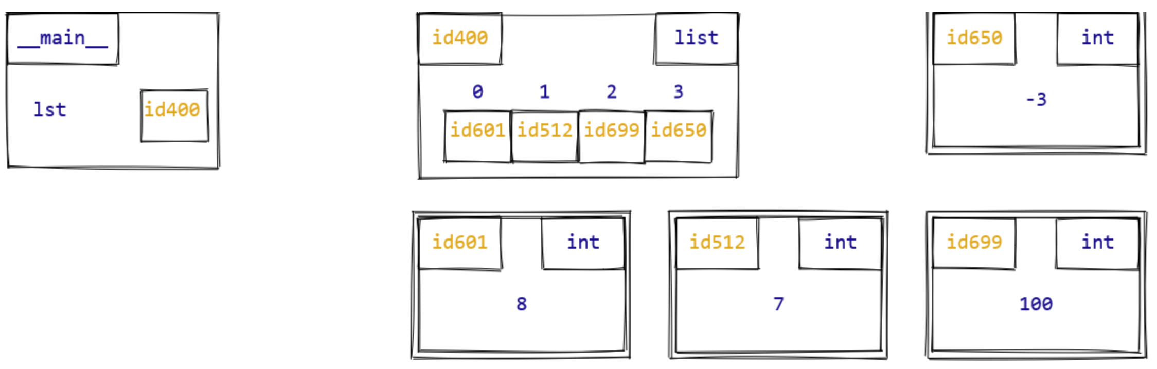
Recall that a Python list object represents an ordered sequence of other objects, which we call its elements. When we studied the object-based memory model in Chapter 6, we drew diagrams like this to represent a list:

Our memory-model diagrams are an abstraction. In reality, all data used by a program are stored in blocks of computer memory, which are labeled by numbers called memory addresses, so that the program can keep track of where each piece of data is stored.

Here is the key idea for how the Python interpreter stores lists in memory. For every Python list object, the references to its elements are stored in a contiguous block of memory. For example, here is how we could picture the same list as in the previous diagram, now stored in blocks of computer memory:

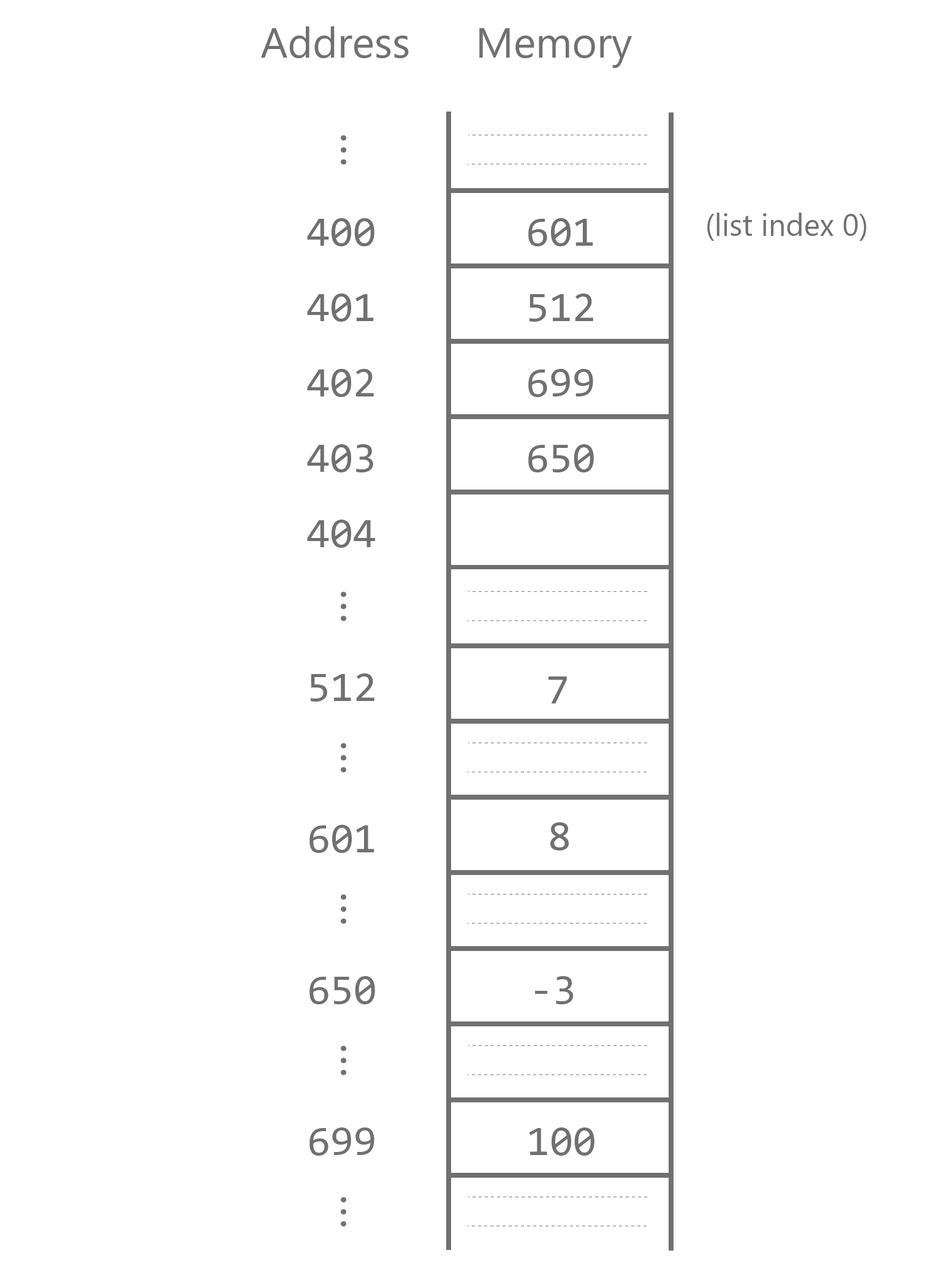
As before, our list stores four integers. In memory, the four consecutive blocks 400–403 store references to the actual integer values. Of course, even this diagram is a simplification of what’s actually going on in computer memory, but it illustrates the main point: the references to each list elements are always stored consecutively. This type of list implementation is used by the Python interpreter and many other programming languages, and is called an array-based list implementation.

Fast list indexing

The primary reason Python uses an array-based list implementation is that it makes list indexing fast. Because the list element references are stored in consecutive memory locations, accessing the i-th element can be done with simple arithmetic: take the memory address where the list starts, and then increase it by i blocks to obtain the the location of the i-th element reference. Think about it like this: suppose you’re walking down a hallway with numbered rooms on just one side and room numbers going up by one. If you see that the first room number is 11, and you’re looking for room 15, you can be confident that it is the fifth room down the hall. More precisely, this means that list indexing is a constant-time operation: its running time does not depend on the size of the list or the index i being accessed. So even with a very long list or a very large index, we expect list indexing to take the same amount of time (and e very fast!).

This is true for both evaluating a list indexing expression or assigning to a list index, e.g. lst[1] = 100. In the latter case, the Python interpreter takes constant time to calculate the memory address where the lst[1] reference is stored and modify it to refer to a new object.

Mutating contiguous memory

Array-based lists have constant time indexing, but as we’ll see again and again in our study of data types, fast operations almost always come at the cost of slow ones. In order for Python to be able to calculate the address of an arbitrary list index, these references must always be stores in a contiguous block of memory; there can’t be any “gaps”.

Maintaining this contiguity has implications for how insertion and deletion in a Python list works. When a list element to be deleted, all items after it have to be moved back one memory block to fill the gap.

Similarly, when a list element is inserted somewhere in the list, all items after it moved forward one block.

In general, suppose we have a list lst of length \(n\) and we wish to remove the element at index \(i\) in the list, where \(0 \leq i < n\). Then \(n - i - 1\) elements must be moved, and the number of “basic operations” this requires is \(\Theta(n - i)\). Here we’re counting moving the contents of one memory block to another as a basic operation. Similarly, if we want to insert an element into a list of length \(n\) at index \(i\), \(n - i\) elements must be moved, and so the running time of this operation is \(\Theta(n - i)\).

At the extremes, this means that inserting/deleting at the front of a Python list (\(i = 0\)) takes \(\Theta(n)\) time, i.e., proportional to the length of list; on the other hand, inserting/deleting at the back of a Python list (\(i = n - 1\)) is a constant-time operation. We can see evidence of this in the following timeit comparisons:

>>> timeit('list.append(lst_1k, 123)', number=10, globals=globals())
1.0400000064691994e-05
>>> timeit('list.append(lst_1m, 123)', number=10, globals=globals())
1.3099999932819628e-05
>>> timeit('list.insert(lst_1k, 0, 123)', number=10, globals=globals())
4.520000015872938e-05
>>> timeit('list.insert(lst_1m, 0, 123)', number=10, globals=globals())
0.011574500000051557

Summary: list mutating method running times

When space runs out

Finally, we should point out one subtle assumption we’ve just made in our analysis of list insertion: that there will always be free memory blocks at the end of the list for the list to expand into. In practice, this is almost always true, and so for the purposes of this course we’ll stick with this assumption. But in CSC263/265 (Data Structures and Analysis), you’ll learn about how programming languages handle array-based list implementations to take into account whether there is “free space” or not, and how these operations still provide the running times we’ve presented in this section.

Running-time analysis with list operations

Now that we’ve learned about the running time of basic list operations, let’s see how to apply this knowledge to analysing the running time of algorithms that use these operations. We’ll look at two different examples.

def squares(numbers: list[int]) -> list[int]:
    """Return a list containing the squares of the given numbers."""
    squares_so_far = []

    for number in numbers:
        list.append(squares_so_far, number ** 2)

    return squares_so_far

In our above analysis, we had to take into account the running of calling list.append, but this quantity did not depend on the length of the input list. Our second example will look very similar to the first, but now we use a different list method that results in a dramatic difference in running time:

def squares_reversed(numbers: list[int]) -> list[int]:
    """Return a list containing the squares of the given numbers, in reverse order."""
    squares_so_far = []

    for number in numbers:
        # Now, insert number ** 2 at the START of squares_so_far
        list.insert(squares_so_far, 0, number ** 2)

    return squares_so_far

To summarize, this single line of code change (from list.append to list.insert at index 0) causes the running time to change dramatically, from \(\Theta(n)\) to \(\Theta(n^2)\). When calling functions and performing operations on data types, we must always be conscious of which functions/operations we’re using and their running times. It is easy to skim over a function call because it takes up so little visual space, but that one call might make the difference between running times of \(\Theta(n)\), \(\Theta(n^2)\), or even \(\Theta(2^n)\)! Lastly, you might be curious how we could speed up squares_reversed. It turns out that Python has a built-in method list.reverse that mutates a list by reversing it, and this method has a \(\Theta(n)\) running time. So we could accumulate the squares by using list.append, and then call list.reverse on the final result.

Sets and dictionaries

It turns out that how Python implements sets and dictionaries is very similar, and so we’ll discuss them together in this section. Both of them are implemented using a more primitive data structure called a hash table, which you’ll also learn about in CSC263/265. The benefit of using hash tables is that they allow constant-time lookup, insertion, and removal of elements (for a set) and key-value pairs (for a dictionary)! This is actually a simplification of how hash tables are implemented. So while we’ll treat all these operations as constant-time in this course, this relies on some technical assumptions which hold in most, but not all, cases.

But of course, there is a catch. The trade-off of how Python uses hash tables is the elements of a set and the keys of a dictionary must all support a “hashing” operation, which the built-in list, set and dict data types do not! This means that in Python, a set cannot contain lists or other sets, for example. This can be inconvenient, but in general is seen as a small price to pay for the speed of their operations.

So if you only care about set operations like “element of”, it is more efficient to use a set than a list: You’ll notice that we haven’t formally discussed the running time of the list in operation in this section. We’ll study it in the next section.

>>> lst1M = list(range(10 ** 6))
>>> set1M = set(range(10 ** 6))
>>> timeit('5000000 in lst1M', number=10, globals=globals())
0.16024739999556914
>>> timeit('5000000 in set1M', number=10, globals=globals())
4.6000059228390455e-06

Data classes

It turns out that data classes (and in fact all Python data types) store their instance attributes using a dictionary that maps attribute names to their corresponding values. This means that data classes benefit from the constant-time dictionary operations that we discussed above.

Explicitly, the two operations that we can perform on a data class instance are looking up an attribute value (e.g., david.age) and mutating the instance by assigning to an attribute (e.g., david.age = 99). Both of these operations take constant time, independent of how many instance attributes the data class has or what values are stored for those attributes.

Aggregation functions

Finally, we’ll briefly discuss a few built-in aggregation functions we’ve seen so far in this course.

sum, max, min have a linear running time (\(\Theta(n)\)), proportional to the size of the input collection. This should be fairly intuitive, as each element of the collection must be processed in order to calculate each of these values.

len is a bit surprising: it has a constant running time (\(\Theta(1)\)), independent of the size of the input collection. In other words, the Python interpreter does not need to process each element of a collection when calculating the collection’s size! Instead, each of these collection data types stores a special attribute referring to the size of that collection. And as we discussed for data classes, accessing attributes takes constant time. There is one technical difference between data class attributes and these collection “size” attributes: we can’t access the latter directly in Python code using dot notation, only through calling len on the collection. This is a result of how the Python language implements these built-in collection data types.