Big-O is a useful way of describing the long-term growth behaviour of functions, but its definition is limited in that it is not required to be an exact description of growth. After all, the key inequality \(g(n) \leq c \cdot f(n)\) can be satisfied even if \(f\) grows much, much faster than \(g\). For example, we could say that \(n + 10 \in \cO(n^{100})\) according to our definition, but this is not necessarily informative.
In other words, the definition of Big-O allows us to express upper bounds on the growth of a function, but does not allow us to distinguish between an upper bound that is tight and one that vastly overestimates the rate of growth.
In this section, we will introduce the final new pieces of notation for this chapter, which allow us to express tight bounds on the growth of a function.
Omega and Theta
Let \(f, g : \N \TO \R^{\ge 0}\). We say that \(g\) is Omega of \(f\) when there exist constants \(c, n_0 \in \R^+\) such that for all \(n \in \N\), if \(n \geq n_0\), then \(g(n) \geq c \cdot f(n)\). In this case, we can also write \(g \in \Omega(f)\).
You can think of Omega as the dual of Big-O: when \(g \in \Omega(f)\), then \(f\) is a lower bound on the growth rate of \(g\). For example, we can use the definition to prove that \(n^2 - n \in \Omega(n)\).
We can now express a bound that is tight for a function’s growth rate quite elegantly by combining Big-O and Omega: if \(f\) is asymptotically both a lower and upper bound for \(g\), then \(g\) must grow at the same rate as \(f\).
Let \(f, g : \N \TO \R^{\ge 0}\). We say that \(g\) is Theta of \(f\) when \(g\) is both Big-O of \(f\) and Omega of \(f\). In this case, we can write \(g \in \Theta(f)\), and say that \(f\) is a tight bound on \(g\).Most of the time, when people say “Big-O” they actually mean Theta, i.e., a Big-O upper bound is meant to be the tight one, because we rarely say upper bounds that overestimate the rate of growth. However, in this course we will always use \(\Theta\) when we mean tight bounds, because we will see some cases where coming up with tight bounds isn’t easy.
Equivalently, \(g\) is Theta of \(f\) when there exist constants \(c_1, c_2, n_0 \in \R^+\) such that for all \(n \in \N\), if \(n \geq n_0\) then \(c_1 f(n) \leq g(n) \leq c_2 f(n)\).
When we are comparing function growth rates, we typically look for a “Theta bound”, as this means that the two functions have the same approximate rate of growth, not just that one is larger than the other. For example, it is possible to prove that \(10n + 5 \in \Theta(n)\), but \(10n + 5 \notin \Theta(n^2)\). Both of these are good exercises to prove, using the above definitions!
A special case: \(\cO(1)\), \(\Omega(1)\), and \(\Theta(1)\)
So far, we have seen Big-O expressions like \(\cO(n)\) and \(\cO(n^2)\), where the function in parentheses has grown to infinity. However, not every function takes on larger and larger values as its input grows. Some functions are bounded, meaning they never take on a value larger than some fixed constant.
For example, consider the constant function \(f(n) = 1\), which always outputs the value \(1\), regardless of the value of \(n\). What would it mean to say that a function \(g\) is Big-O of this \(f\)? Let’s unpack the definition of Big-O to find out.
\[\begin{align*} & g \in \cO(f) \\ & \exists c, n_0 \in \R^+,~ \forall n \in \N,~ n \geq n_0 \IMP g(n) \leq c \cdot f(n) \\ & \exists c, n_0 \in \R^+,~ \forall n \in \N,~ n \geq n_0 \IMP g(n) \leq c \tag{since $f(n) = 1$} \end{align*}\]
In other words, there exists a constant \(c\) such that \(g(n)\) is eventually always less than or equal to \(c\). We say that such functions \(g\) are asymptotically bounded with respect to their input, and write \(g \in \cO(1)\) to represent this.
Similarly, we use \(g \in \Omega(1)\) to express that functions are greater than or equal to some constant \(c\). You might wonder why we would ever say this—don’t all functions satisfy this property? While the functions we’ll be studying in later chapters in this section are generally going to be \(\geq 1\), this is not true for all mathematical functions. For example, the function \(g(n) = \frac{1}{n + 1}\) is \(\cO(1)\), but not \(\Omega(1)\). More generally, any function \(g\) where \(\lim_{n \to \infty} g(n) = 0\) is not \(\Omega(1)\).
On the other hand, the function \(g(n) = n^2\) is \(\Omega(1)\) but not \(\cO(1)\). So we reserve \(\Theta(1)\) to refer to the functions that are both \(\cO(1)\) and \(\Omega(1)\).
Properties of Big-O, Omega, and Theta
If we had you always write chains of inequalities to prove that one function is Big-O/Omega/Theta of another, that would get quite tedious rather quickly. Instead, in this section we will prove some properties of this definition which are extremely useful for combining functions together under this definition. These properties can save you quite a lot of work in the long run. We’ll illustrate the proof of one of these properties here; most of the others can be proved in a similar manner, while a few are most easily proved using some techniques from calculus.We discuss the connection between calculus and asymptotic notation in the following section, but this is not a required part of CSC110.
Elementary functions
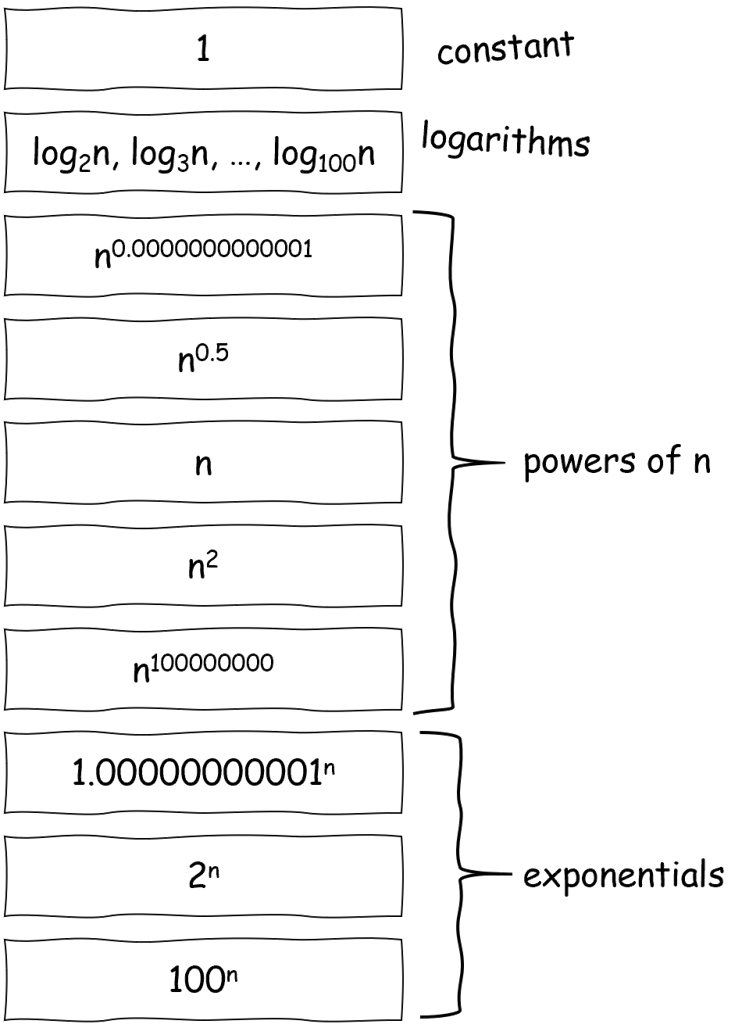
The following theorem tells us how to compare four different types of “elementary” functions: constant functions, logarithms, powers of \(n\), and exponential functions.
(Elementary function growth hierarchy theorem.)
For all \(a, b \in \R^+\), the following statements are true:
- If \(a > 1\) and \(b > 1\), then \(\log_a n \in \Theta(\log_b n)\).
- If \(a < b\), then \(n^a \in \cO(n^b)\) and \(n^a \notin \Omega(n^b)\).
- If \(a < b\), then \(a^n \in \cO(b^n)\) and \(a^n \notin \Omega(b^n)\).
- If \(a > 1\), then \(1 \in \cO(\log_a n)\) and \(1 \notin \Omega(\log_a n)\).
- \(\log_a n \in \cO(n^b)\) and \(\log_a n \notin \Omega(n^b)\).
- If \(b > 1\), then \(n^a \in \cO(b^n)\) and \(n^a \notin \Omega(b^n)\).
And here is a handy figure to show the progression of functions toward larger and larger rates of growth:
Basic properties
Now, here are three properties of Big-O, Omega, and Theta that apply to all functions. We won’t prove these statements here, but you should be able to prove each of them from just definitions alone!
For all \(f : \N \to \R^{\geq 0}\), \(f \in \Theta(f)\). (Note that this also implies that \(f \in \cO(f)\) and \(f \in \Omega(f)\).)
For all \(f, g : \N \to \R^{\geq 0}\), \(g \in \cO(f)\) if and only if \(f \in \Omega(g)\).As a consequence of this, \(g \in \Theta(f)\) if and only if \(f \in \Theta(g)\).
For all \(f, g, h : \N \to \R^{\geq 0}\):
- If \(f \in \cO(g)\) and \(g \in \cO(h)\), then \(f \in \cO(h)\).
- If \(f \in \Omega(g)\) and \(g \in \Omega(h)\), then \(f \in \Omega(h)\).
- If \(f \in \Theta(g)\) and \(g \in \Theta(h)\), then \(f \in \Theta(h)\).
Operations on functions
Let \(f, g : \N \TO \R^{\ge 0}\). We can define the sum of \(f\) and \(g\) as the function \(f + g : \N \TO \R^{\ge 0}\) such that \[\forall n \in \N,~ (f + g)(n) = f(n) + g(n).\]
For all \(f, g, h : \N \to \R^{\geq 0}\), the following hold:
- If \(f \in \cO(h)\) and \(g \in \cO(h)\), then \(f + g \in \cO(h)\).
- If \(f \in \Omega(h)\), then \(f + g \in \Omega(h)\).
- If \(f \in \Theta(h)\) and \(g \in \cO(h)\), then \(f + g \in \Theta(h)\). Exercise: prove this using the first two.
We’ll prove the first of these statements.
\[\forall f, g, h : \N \TO \R^{\ge 0},~ \big(f \in \cO(h) \AND g \in \cO(h)\big) \IMP f + g \in \cO(h).\]
This is similar in spirit to the divisibility proofs we did back in 4.6 Proofs and Programming I: Divisibility, which used a term (divisibility) that contained a quantifier.The definition of Big-O here has three quantifiers, but the idea is the same. Here, we need to assume that \(f\) and \(g\) are both Big-O of \(h\), and prove that \(f + g\) is also Big-O of \(h\).
Assuming \(f \in \cO(h)\) tells us there exist positive real numbers \(c_1\) and \(n_1\) such that for all \(n \in \N\), if \(n \geq n_1\) then \(f(n) \leq c_1 \cdot h(n)\). There similarly exist \(c_2\) and \(n_2\) such that \(g(n) \leq c_2 \cdot h(n)\) whenever \(n \geq n_2\). Warning: we can’t assume that \(c_1 = c_2\) or \(n_1 = n_2\), or any other relationship between these two sets of variables.
We want to prove that there exist \(c, n_0 \in \R^+\) such that for all \(n \in \N\), if \(n \geq n_0\) then \(f(n) + g(n) \leq c \cdot h(n)\).
The forms of the inequalities we can assume—\(f(n) \leq c_1 h(n)\), \(g(n) \leq c_2 h(n)\)—and the final inequality are identical, and in particular the left-hand side suggests that we just need to add the two given inequalities together to get the third. We just need to make sure that both given inequalities hold by choosing \(n_0\) to be large enough, and let \(c\) be large enough to take into account both \(c_1\) and \(c_2\).
Let \(f, g, h : \N \TO \R^{\ge 0}\), and assume \(f \in \cO(h)\) and \(g \in \cO(h)\). By these assumptions, there exist \(c_1, c_2, n_1, n_2 \in \R^+\) such that for all \(n \in \N\),
- if \(n \geq n_1\), then \(f(n) \leq c_1 \cdot h(n)\), and
- if \(n \geq n_2\), then \(g(n) \leq c_2 \cdot h(n)\).
We want to prove that \(f + g \in \cO(h)\), i.e., that there exist \(c, n_0 \in \R^+\) such that for all \(n \in \N\), if \(n \geq n_0\) then \(f(n) + g(n) \leq c \cdot h(n)\).
Let \(n_0 = \max \{n_1, n_2\}\) and \(c = c_1 + c_2\). Let \(n \in \N\), and assume that \(n \geq n_0\). We now want to prove that \(f(n) + g(n) \leq c \cdot h(n)\).
Since \(n_0 \geq n_1\) and \(n_0 \geq n_2\), we know that \(n\) is greater than or equal to \(n_1\) and \(n_2\) as well. Then using the Big-O assumptions, \[\begin{align*} f(n) &\leq c_1 \cdot h(n) \\ g(n) &\leq c_2 \cdot h(n) \end{align*}\]
Adding these two inequalities together yields
\[f(n) + g(n) \leq c_1 h(n) + c_2 h(n) = (c_1 + c_2) h(n) = c \cdot h(n).\]
For all \(f : \N \to \R^{\geq 0}\) and all \(a \in \R^+\), \(a \cdot f \in \Theta(f)\).
For all \(f_1, f_2, g_1, g_2 : \N \to \R^{\geq 0}\), if \(g_1 \in \cO(f_1)\) and \(g_2 \in \cO(f_2)\), then \(g_1 \cdot g_2 \in \cO(f_1 \cdot f_2)\). Moreover, the statement is still true if you replace Big-O with Omega, or if you replace Big-O with Theta.
For all \(f : \N \to \R^{\geq 0}\), if \(f(n)\) is eventually greater than or equal to \(1\), then \(\floor{f} \in \Theta(f)\) and \(\ceil{f} \in \Theta(f)\).