In the previous section, we began our study of program running time with a few simple examples to guide our intuition. One question that emerged from these examples was how we define what “basic operations” we actually count when analyzing a program’s running time—or better yet, how we can ignore small differences in counts that result from slightly different definitions of “basic operation”. This question grows even more important as we study more complex algorithms consisting of many lines of code.
Over the next two sections, we’ll develop a powerful mathematical tool for comparing function growth rates. This will formalize the idea of “linear”, “quadratic”, “logarithmic”, and “constant” running times from the previous section, and extend these categories to all types of functions.
Four kinds of dominance
Here is a quick reminder about function notation. When we write \(f : A \to B\), we say that \(f\) is a function which maps elements of \(A\) to elements of \(B\). In this chapter, we will mainly be concerned about functions mapping the natural numbers to the non-negative real numbers,These are the domain and codomain which arise in algorithm analysis—an algorithm can’t take “negative” time to run, after all. i.e., functions \(f: \N \to \R^{\geq 0}\). Though there are many different properties of functions that mathematicians study, we are only going to look at one such property: describing the long-term (i.e., asymptotic) growth of a function. We will proceed by building up a few different definitions of comparing function growth, which will eventually lead into one which is robust enough to be used in practice.
Let \(f, g : \N \to \R^{\ge 0}\). We say that \(g\) is absolutely dominated by \(f\) when for all \(n \in \N\), \(g(n) \leq f(n)\).
Let \(f(n) = n^2\) and \(g(n) = n\). Prove that \(g\) is absolutely dominated by \(f\).
This is a straightforward unpacking of a definition, which you should be very comfortable with by now: \(\forall n \in \N,~ g(n) \leq f(n)\).Note that we aren’t quantifying over \(f\) and \(g\); the “let” in the example defines concrete functions that we want to prove something about.
Let \(n \in \N\). We want to show that \(n \leq n^2\).
Case 1: Assume \(n = 0\). In this case, \(n^2 = n = 0\), so the inequality holds.
Case 2: Assume \(n \geq 1\). In this case, we take the inequality \(n \geq 1\) and multiply both sides by \(n\) to get \(n^2 \geq n\), or equivalently \(n \leq n^2.\)
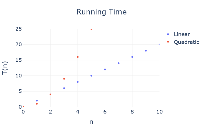
Unfortunately, absolute dominance is too strict for our purposes: if \(g(n) \leq f(n)\) for every natural number except \(5\), then we can’t say that \(g\) is absolutely dominated by \(f\). For example, the function \(g(n) = 2n\) is not absolutely dominated by \(f(n) = n^2\), even though \(g(n) \leq f(n)\) everywhere except \(n = 1\). Graphically:
Here is another definition which is a bit more flexible than absolute dominance.
Let \(f, g : \N \to \R^{\ge 0}\). We say that \(g\) is dominated by \(f\) up to a constant factor when there exists a positive real number \(c\) such that for all \(n \in \N\), \(g(n) \leq c \cdot f(n)\).
Let \(f(n) = n^2\) and \(g(n) = 2n\). Prove that \(g\) is dominated by \(f\) up to a constant factor.
Once again, the translation is a simple unpacking of the previous definition:Remember: the order of quantifiers matters! The choice of \(c\) is not allowed to depend on \(n\).
\[\exists c \in \R^+,~ \forall n \in \N,~ g(n) \leq c \cdot f(n).\]
The term “constant factor” is revealing. We already saw that \(n\) is absolutely dominated by \(n^2\), so if the \(n\) is multiplied by \(2\), then we should be able to multiply \(n^2\) by \(2\) as well to get the calculation to work out.
Let \(c = 2\), and let \(n \in \N\). We want to prove that \(g(n) \leq c \cdot f(n)\), or in other words, \(2n \leq 2n^2\).
Case 1: Assume \(n = 0\). In this case, \(2n = 0\) and \(2n^2 = 0\), so the inequality holds.
Case 2: Assume \(n \geq 1\). In this case, we can take this inequality and multiply both sides by \(2n\) to obtain \(2n^2 \geq 2n\), or equivalently \(2n \leq 2n^2\).
Intuitively, “dominated by up to a constant factor” allows us to ignore multiplicative constants in our functions. This will be very useful in our running time analysis because it frees us from worrying about the exact constants used to represent numbers of basic operations: \(n\), \(2n\), and \(11n\) are all equivalent in the sense that each one dominates the other two up to a constant factor.
However, this second definition is still a little too restrictive, as the inequality must hold for every value of \(n\). Consider the functions \(f(n) = n^2\) and \(g(n) = n + 90\). No matter how much we scale up \(f\) by multiplying it by a constant, \(f(0)\) will always be less than \(g(0)\), so we cannot say that \(g\) is dominated by \(f\) up to a constant factor. And again this is silly: it is certainly possible to find a constant \(c\) such that \(g(n) \leq cf(n)\) for every value except \(n = 0\). So we want some way of omitting the value \(n = 0\) from consideration; this is precisely what our third definition gives us.
Let \(f, g : \N \to \R^{\ge 0}\). We say that \(g\) is eventually dominated by \(f\) when there exists \(n_0 \in \R^+\) such that \(\forall n \in \N\), if \(n \geq n_0\) then \(g(n) \leq f(n)\).
Let \(f(n) = n^2\) and \(g(n) = n + 90\). Prove that \(g\) is eventually dominated by \(f\).
\[\exists n_0 \in \R^+,~ \forall n \in \N,~ n \geq n_0 \Rightarrow g(n) \leq f(n).\]
Okay, so rather than finding a constant to scale up \(f\), we need to argue that for “large enough” values of \(n\), \(n + 90 \leq n^2\). How do we know that value of \(n\) is “large enough?”
Since this is a quadratic inequality, it is actually possible to solve it directly using factoring or the quadratic formula. But that’s not really the point of this example, so instead we’ll take advantage of the fact that we get to choose the value of \(n_0\) to pick one which is large enough.
Let \(n_0 = 90\), let \(n \in \N\), and assume \(n \geq n_0\). We want to prove that \(n + 90 \leq n^2\).
We will start with the left-hand side and obtain a chain of inequalities that lead to the right-hand side. \[\begin{align*} n + 90 &\leq n + n \tag{since $n \geq 90$} \\ &= 2n \\ &\leq n \cdot n \tag{since $n \geq 2$} \\ &= n^2 \end{align*}\]
Intuitively, this definition allows us to ignore “small” values of \(n\) and focus on the long term, or asymptotic, behaviour of the function. This is particularly important for ignoring the influence of slow-growing terms in a function, which may affect the function values for “small” \(n\), but eventually are overshadowed by the faster-growing terms. In the above example, we knew that \(n^2\) grows faster than \(n\), but because an extra \(+ 90\) was added to the latter function, it took a while for the faster growth rate of \(n^2\) to “catch up” to \(n + 90\).
Our final definition combines both of the previous ones, enabling us to ignore both constant factors and small values of \(n\) when comparing functions.
Let \(f, g: \N \to \R^{\ge 0}\). We say that \(g\) is eventually dominated by \(f\) up to a constant factor when there exist \(c, n_0 \in \R^+\), such that for all \(n \in \N\), if \(n \geq n_0\) then \(g(n) \leq c \cdot f(n)\).
In this case, we also say that \(g\) is Big-O of \(f\), and write \(g \in \cO(f)\).
We use the notation “\(\in \cO(f)\)” here because we formally define \(\cO(f)\) to be the set of functions that are eventually dominated by \(f\) up to a constant factor: \[\cO(f) = \{g \mid g: \N \to \R^{\ge 0},~\text{and}~\exists c, n_0 \in \R^+,~ \forall n \in \N,~ n \geq n_0 \Rightarrow g(n) \leq c \cdot f(n)\}.\]
Let \(f(n) = n^3\) and \(g(n) = n^3 + 100n + 5000\). Prove that \(g \in \cO(f)\).We can also express this statement as “\(n^3 + 100n + 5000 \in \cO(n^3)\)”.
\[\exists c, n_0 \in \R^+,~ \forall n \in \N,~ n \geq n_0 \Rightarrow n^3 + 100n + 5000 \leq c n^3.\]
It’s worth pointing out that in this case, \(g\) is neither eventually dominated by \(f\) nor dominated by \(f\) up to a constant factor. Exercise: prove this! So we’ll really need to make use of both constants \(c\) and \(n_0\). They’re both existentially-quantified, so we have a lot of freedom in how to choose them!
Here’s an idea: let’s split up the inequality \(n^3 + 100n + 5000 \leq c n^3\) into three simpler ones: \[\begin{align*} n^3 &\leq c_1 n^3 \\ 100n &\leq c_2 n^3 \\ 5000 &\leq c_3 n^3 \end{align*}\]
If we can make these three inequalities true, adding them together will give us our desired result (setting \(c = c_1 + c_2 + c_3\)). Each of these inequalities is simple enough that we can “solve” them by inspection. Moreover, because we have freedom in how we choose \(n_0\) and \(c\), there are many different ways to satisfy these inequalities! To illustrate this, we’ll look at two different approaches here.
Approach 1: focus on choosing \(n_0\).
It turns out we can satisfy the three inequalities even if \(c_1 = c_2 = c_3 = 1\):
- \(n^3 \leq n^3\) is always true (so for all \(n \geq 0\)).
- \(100n \leq n^3\) when \(n \geq 10\).
- \(5000 \leq n^3\) when \(n \geq \sqrt[3]{5000} \approx 17.1\)
We can pick \(n_0\) to be the largest of the lower bounds on \(n\), \(\sqrt[3]{5000}\), and then these three inequalities will be satisfied!
Approach 2: focus on choosing \(c\).
Another approach is to pick \(c_1\), \(c_2\), and \(c_3\) to make the right-hand sides large enough to satisfy the inequalities.
- \(n^3 \leq c_1 n^3\) when \(c_1 = 1\).
- \(100n \leq c_2 n^3\) when \(c_2 = 100\).
- \(5000 \leq c_3 n^3\) when \(c_3 = 5000\), as long as \(n \geq 1\).
(Using Approach 1) Let \(c = 3\) and \(n_0 = \sqrt[3]{5000}\). Let \(n \in \N\), and assume that \(n \geq n_0\). We want to show that \(n^3 + 100n + 5000 \leq c n^3\).
First, we prove three simpler inequalities:
- \(n^3 \leq n^3\) (since the two quantities are equal).
- Since \(n \geq n_0 \geq 10\), we know that \(n^2 \geq 100\), and so \(n^3 \geq 100n\).
- Since \(n \geq n_0\), we know that \(n^3 \geq n_0^3 = 5000\).
Adding these three inequalities gives us: \[n^3 + 100n + 5000 \leq n^3 + n^3 + n^3 = c n^3.\]
(Using Approach 2) Let \(c = 5101\) and \(n_0 = 1\). Let \(n \in \N\), and assume that \(n \geq n_0\). We want to show that \(n^3 + 100n + 5000 \leq c n^3\).
First, we prove three simpler inequalities:
- \(n^3 \leq n^3\) (since the two quantities are equal).
- Since \(n \in \N\), we know that \(n \leq n^3\), and so \(100n \leq 100n^3\).
- Since \(1 \leq n\), we know that \(1 \leq n^3\), and then multiplying both sides by 5000 gives us \(5000 \leq 5000n^3\).
Adding these three inequalities gives us: \[n^3 + 100n + 5000 \leq n^3 + 100n^3 + 5000n^3 = 5101 n^3 = c n^3.\]
Summary
In this section, we covered four definitions used to compare two functions. The first, absolute dominance, is the strictest, stating that \(g(n) \leq f(n)\) for every value of \(n \in \N\). We then learned about two different relaxations of dominance: “dominance up to a constant factor”, which allows us to scale up \(f(n)\) by multiplying it by a constant, and “eventual dominance”, which allows us to ignore small values of \(n\) when comparing the two functions.
The last and most important definition in this section combined these two relaxations into a single definition: \(g \in \cO(f)\) means that “\(g\) is eventually dominated by \(f\) up to a constant factor”. The symbolic form of this definition is one of the most complex mathematical definitions we’ve studied in this course so far:
\[ g \in \cO(f): \exists c, n_0 \in \R^+,~ \forall n \in \N,~ n \geq n_0 \Rightarrow g(n) \leq c \cdot f(n) \]
Please take a moment to review it and the example proof of a Big-O statement to solidify your understanding before moving onto the next section!