So far in this course, when we have studied programming concepts, we have focused on the correctness of our code. In Chapters 1–6, we learned about different programming constructs, understanding what they do, how to combine them into larger programs, and how to test these programs to make sure they are correct. In Chapters 7 and 8, we learned about the mathematical domain of number theory, and applied our learning to prove the correctness of various algorithms, including the famed RSA cryptosystem.
Yet when it comes to evaluating programs, correctness is not the only important measure. As we alluded to in Chapter 8, the amount of time a program takes to run, or program running time, is a critical consideration. Running time is often shortened to “runtime”, and is also known as the “efficiency” or “performance” of a program. In this chapter, we’ll study a formal approach to analyzing the running time of a program. This section will introduce the topic, and then in future sections we’ll build up some mathematical theory about comparing rates of function growth, and then apply this theory to real program code.
How do we measure running time?
Consider the following function, which prints out the first
n natural numbers:
def print_integers(n: int) -> None:
    for i in range(0, n):
        print(i)
What can we say about the running time of this function? An empirical approach would be to measure the time it takes for this function to run on a bunch of different inputs, and then take the average of these times to come up with some sort of estimate of the “average” running time.
But of course, given that this algorithm performs an action for every
natural number between 0 and n - 1, we expect
it to take longer as n gets larger, so taking an average of
a bunch of running times loses important information about the
inputs.This is like doing a random poll of how many birthday
cakes people have eaten without taking into account how old the
respondents are.
How about choosing one particular input, calling the function multiple times on that input, and averaging those running times? This seems better, but even here there are some problems. For one, the computer’s hardware can affect running time; for another, computers all are running multiple programs at the same time, so what else is currently running on your computer also affects running time. So even running this experiment on one computer wouldn’t necessarily be indicative of how long the function would take on a different computer, nor even how long it would take on the same computer running a different number of other programs.
While these sorts of timing experiments are actually done in practice for evaluating particular hardware or extremely low-level (close to hardware) programs, these details are often not helpful for most software developers, as they do not have control over the machine on which their software will be run. That said, these timing experiments can provide an intuitive understanding of the efficiency of our programs. We will explore how to conduct basic timing experiments at the end of this chapter.
So rather than use an empirical measurement of runtime, what we do instead is use an abstract representation of runtime: the number of “basic operations” an algorithm executes. This means that we can analyze functions without needing a computer, and our analysis theoretically applies to any computer system. However, there is a good reason “basic operation” is in quotation marks—this vague term raises a whole slew of questions:
- What counts as a “basic operation”?
- How do we tell which “basic operations” are used by an algorithm?
- Do all “basic operations” take the same amount of time?
The answers to these questions can depend on the hardware being used,
as well as what programming language the algorithm is written in. Of
course, these are precisely the details we wish to avoid thinking about.
In this section, we will count only the calls to print as
basic operations, and study print_integers and some
variations to establish some intuition and terminology.
Linear running time
First, let’s return to print_integers.
def print_integers(n: int) -> None:
    for i in range(0, n):
        print(i)
From Chapter 5, we know that the for loop will call
print once per iteration. We also know that this loop
iterates \(n\) times (with
i taking on the values 0, 1, 2, …, \(n - 1\)):
>>> print_integers(2)
0
1
>>> print_integers(4)
0
1
2
3
>>> print_integers(8)
0
1
2
3
4
5
6
7
So then for an input \(n\), there
are \(n\) calls to print.
We say that the running time of print_integers on input
\(n\) is \(n\) basic operations. If we plot \(n\) against this measure running time, we
obtain a line:
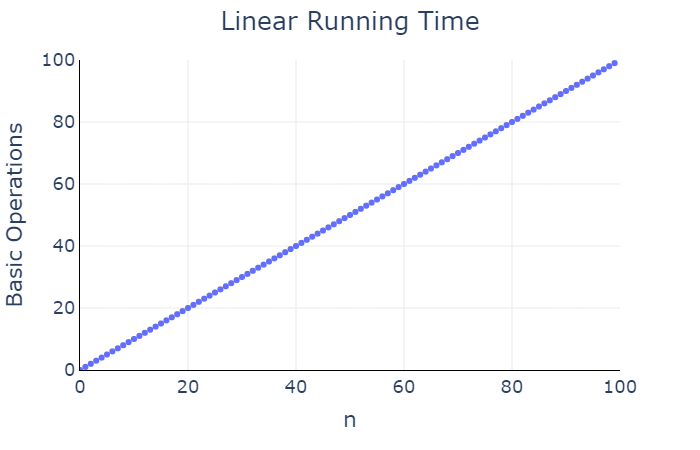
We say that print_integers has a linear
running time, as the number of basic operations is a linear function of
the input \(n\).
Quadratic running time
Let us now consider a function that prints all combinations of pairs of integers:
def print_pairs(n: int) -> None:
    """Print all combinations of pairs of the first n natural numbers."""
    for i in range(0, n):
        for j in range(0, n):
            print(i, j)
What is the running time of this function? Similar to our previous
example, there is a for loop that calls print \(n\) times, but now this loop is nested
inside another for loop. Let’s see some examples of this function being
called:
>>> print_pairs(1)
0 0
>>> print_pairs(2)
0 0
0 1
1 0
1 1
>>> print_pairs(3)
0 0
0 1
0 2
1 0
1 1
1 2
2 0
2 1
2 2
If we look at the outer loop (loop variable i), we see
that it repeats its body \(n\) times.
But its body is another loop, which repeats its body \(n\) times. So the inner loop takes \(n\) calls to print each time it is
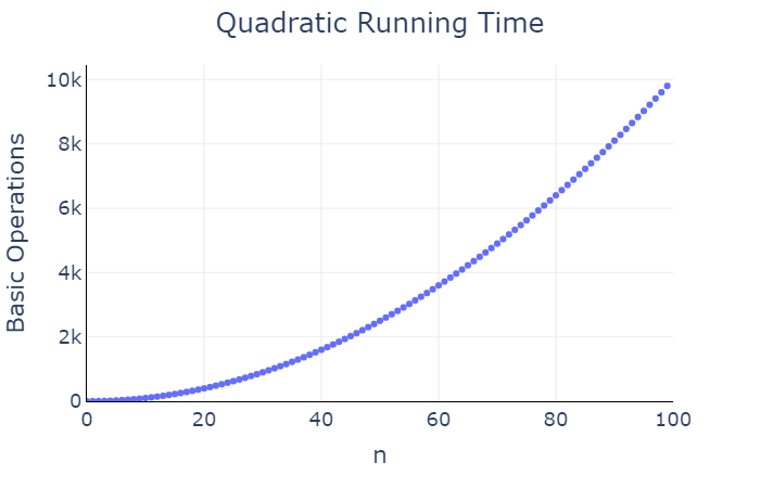
executed, and it is executed \(n\)
times in total. This means print is called \(n^2\) times in total.
We say that print_pairs has a quadratic
running time, as the number of basic operations is a quadratic function
of the input \(n\).
Logarithmic running time
Now let’s consider the following function, which prints out the powers of two that are less than a positive integer \(n\). These numbers are of the form \(2^i\), where \(i\) can range from 0 to \(\ceil{\log_2(n)} - 1\). For example, when \(n = 16\), \(\ceil{\log_2(n)} = 4\), and \(i\) ranges from 0 to 3. When \(n = 7\), \(\ceil{\log_2(n)} = 3\), and \(i\) ranges from 0 to 2.
import math
def print_powers_of_two(n: int) -> None:
"""Print the powers of two that are less than n.
Preconditions:
- n > 0
"""
for i in range(0, math.ceil(math.log2(n))):
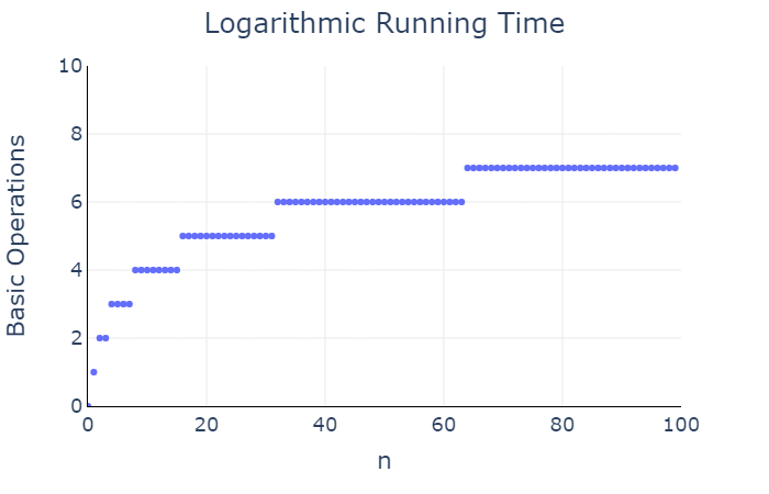
print(2 ** i)In this case, the number of calls to print is \(\ceil{\log_2(n)}\). So the running time of
print_powers_of_two is approximately, but not
exactly, \(\log_2(n)\). Yet in this
case we still say that print_powers_of_two has a
logarithmic running time.
Constant running time
Our final example in this section is a bit unusual.
def print_ten(n: int) -> None:
"""Print n ten times."""
for i in range(0, 10):
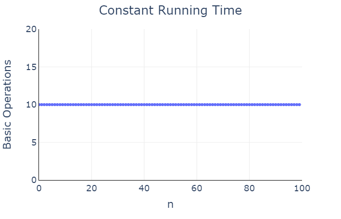
print(n)How many times is print called here? We can again tell
from the header of the for loop: this loop iterates 10 times, and so
print is called 10 times, regardless of what \(n\) is!
We say that print_ten has a constant
running time, as the number of basic operations is independent to the
input size.
Basic operations
In the past four examples, we have seen examples of functions that have linear, quadratic, logarithmic, and constant running times. While these labels are not precise, they do give us intuition about the relative size of each function.
Functions with linear running time are faster than ones with quadratic running time, and slower than ones with logarithmic running time. Functions with a constant running time are the fastest of all.
But all of our informal analyses in the previous section relied on
defining a “basic operation” to be a call to print. We
said, for example, that the running time of print_integers
had a running time of \(n\). But what
if we had a friend comes along and say, “No wait, the variable
i must be assigned a new value at every loop iteration, and
that counts as a basic operation.” Okay, so then we would say that there
are \(n\) print calls and
\(n\) assignments to i,
for a total running time of \(2n\)
basic operations for an input \(n\).
But then another friend chimes in, saying “But print
calls take longer than variable assignments, since they need to change
pixels on your monitor, so you should count each print call
as \(10\) basic operations.” Okay, so
then there are \(n\) print calls worth
\(10n\) basic operations, plus the
assignments to i, for a total of \(11n\) basic operations for an input \(n\).
And then another friend joins in: “But you need to factor in an
overhead of calling the function as a first step before the body
executes, which counts as \(1.5\) basic
operations (slower than assignment, faster than print).” So
then we now have a running time of \(11n +
1.5\) basic operations for an input \(n\).
And then another friend starts to speak, but you cut them off and say “That’s it! This is getting way too complicated. I’m going back to timing experiments, which may be inaccurate but at least I won’t have to listen to these increasing levels of fussiness.”
The expressions \(n\), \(2n\), \(11n\), and \(11n + 1.5\) may be different mathematically, but they share a common qualitative type of growth: they are all linear. And so we know, at least intuitively, that they are all faster than quadratic running times and slower than logarithmic running times. What we will study in the next section is how to make this observation precise, and thus avoid the tedium of trying to exactly quantify our “basic operations”, and instead measure the overall rate of growth in the number of operations.
References
- CSC108 video: Algorithm Analysis