In the previous section, we discussed one way that variables can “change value” during the execution of a Python program. In this section, we’ll introduce the other way values can change, a phenomenon called object mutation. But to understand how object mutation happens, we’re first going to need to go a bit deeper into precisely how the Python interpreter stores data.
Objects and the Python data model
Up to this point in our study of the Python programming language, we’ve talked about representing data in terms of values that actually contain the data and variables that are names that refer to values. This has been a useful simplification when learning the fundamentals of programming in Python, but we’re ready now to go further.
In Python, every piece of data is stored in an entity called an object. Every object has three fundamental components: its id, its data type, and its value. A useful metaphor here is to view an object as a box: the object’s id and type are like labels printed on the box, and the value is some piece of data that’s stored inside the box. In the past when we’ve talked about “values” in a Python program, we’ve really been talking about “objects that contain values”. And when we’ve talked about the data type of a particular value, we’re really been talking about the data type of the object that contains the value.
But what is the id of an object, really? To understand this
component, let’s think about how data is stored in your computer. Every
computer program (whether written in Python or some other language)
stores data in computer memory, which you can think of as a very long
list of storage locations, each with a unique memory
address. This is analogous to a very long street, with each
building having a unique number as its street address. In Python,
every object we use is stored in computer memory at a particular
location, and it is the responsibility of the Python interpreter to keep
track of which objects are stored at which memory locations. Formally,
the id of an object is a unique int
representation of the memory address of the object. As Python
programmers, we cannot control or modify which memory address is used to
store a given object, but we can access the id of an object using the
built-in id function:
>>> id(3)
1635361280
>>> id('words')
4297547872
Okay, so that’s objects, ids, types, and values. But you might be wondering, why are talking about this? Here is the fundamental property that’s relevant to our discussion this chapter: once an object its created, its id and type can never change, but (depending on the data type), its value may change. To use our earlier analogy, once the Python interpreter has created a “box” to store some data, the labels on the box can’t change, but the contents of the box can (sometimes) change. This is the other form of “value change” in a Python program, called object mutation.
Object mutation
In 5.7 Nested
Loops, we saw how cartesian_product could help us
calculate the Cartesian product by accumulating all possible pairs of
elements in a list. Now, let’s consider a similar function that
accumulates values in a list:
def squares(nums: list[int]) -> list[int]:
    """Return a list of the squares of the given numbers.

    >>> squares([1, 2, 3])
    [1, 4, 9]
    """
    squares_so_far = []

    for num in nums:
        squares_so_far = squares_so_far + [num * num]
    return squares_so_far
Both squares and cartesian_product
functions are implemented correctly, but are rather
inefficient. We’ll study what we mean by “inefficient” more
precisely later in this course. In squares, each
loop iteration creates a new list object (a copy of the
current list plus one more element at the end) and reassigns
squares_so_far to it. It would be easier (and faster) if we
could somehow reuse the same object but modify it by adding elements to
it; the same applies to other collection data types like
set and dict as well.
In Python, object mutation (often shortened to just
mutation) is an operation that changes the value of an
existing object. For example, Python’s list data type
contains several methods that mutate the given
list object rather than create a new one. Here’s how we
could improve our squares implementation by using
list.append,Check out Appendix A.2 Python Built-In
Data Types Reference for a list of methods, including mutating ones,
for lists, sets, dictionaries, and more. a method that adds a
single value to the end of a list:
def squares(nums: list[int]) -> list[int]:
    """Return a list of the squares of the given numbers.

    >>> squares([1, 2, 3])
    [1, 4, 9]
    """
    squares_so_far = []

    for num in nums:
        squares_so_far.append(num * num)
    return squares_so_far
Now, squares runs by assigning
squares_so_far to a single list object before the loop, and
then mutating that list object at each loop iteration. The outward
behaviour is the same, but this code is more efficient because a bunch
of new list objects are not created. To use the terminology from before,
squares_so_far is not reassigned; instead, the
object that it refers to gets mutated.
One final note: you might notice that the loop body calls
squares_so_far.append without an assignment statement. This
is because the list.append method returns
None, a special Python value that indicates “no value”.
Just as we explored previously with the print function,
list.append has a side effect that it mutates its
list argument, but does not return anything.
Variable reassignment vs. object mutation
We have now seen both variable reassignment and object mutation, let
us take a moment to examine the similarities and differences between the
two. We can use as inspiration our two different versions of
squares, which illustrated these two forms of “value
change”. Let’s extract out the relevant part and look at it in more
detail in the Python console. Suppose we have a variable
squares_so_far = [1, 4, 9] and want to add 16
to the end of it. We can do this through either variable reassignment or
object mutation, as shown in the table below.
| Variable reassignment version | Object mutation version |
|---|---|
First, create the new variable. |
First, create the new variable. |
Then reassign the variable. |
Then mutate the object that the variable refers to. |
By just looking at the final value of squares_so_far, it
seems like the variable reassignment version and object mutation version
had the same effect. Yet we claimed above that the object mutation
version was “faster” because it didn’t need to create a copy of the new
list. How can we tell this actually happens?
One way is to use the id function to inspect the ids of
the objects that squares_so_far refers to at each step in
the process. Let’s modify our example to call
id(squares_so_far) at each step.
| Variable reassignment version | Object mutation version |
|---|---|
First, create the new variable. |
First, create the new variable. |
Then reassign the variable. |
Then mutate the object that the variable refers to. |
Of course, the specific id values shown are just
examples, and will differ on your computer. The important part is that
in the variable reassignment version, the id values are
different before and after the reassignment. This is consistent with
what we said above: the statement
squares_so_far = squares_so_far + [16] creates a new
list object and assigns that to squares_so_far, and
every object has a unique id. On the other hand, in the object mutation
version the ids are the same before and after the mutation operation.
squares_so_far continues to refer to the same list object,
but the value of that object has changed as a result of the
mutation.
Reasoning about code with changing values
Even though variable reassignment and object mutation are distinct concepts, they share a fundamental similarity: they both result in variables changing values over the course of a program. So far we’ve focused on individual lines of code, but let’s now take a step back and consider the implications of “changing values over the course of a program”. Consider the following hypothetical function definition:
def my_function(...) -> ...:
    x = 10
    y = [1, 2, 3]

    ...  # Many lines of code
    ...  # Many lines of code
    ...  # Many lines of code
    ...  # Many lines of code
    ...  # Many lines of code
    ...  # Many lines of code

    return x * len(y) + ...
We’ve included for effect a large omitted “middle” section of the function body, showing only the initialization of two local variables at the start of the function and a final return statement at the end of the function.
If the omitted code does not contain any variable
reassignment or object mutation, then we can be sure that in the return
statement, x still refers to 10 and
y still refers to [1, 2, 3], regardless of
what other computations occurred in the omitted lines! In other words,
without reassignment and mutation, these assignment statements are
universal across the function body: “for all points in the body of
my_function, x == 10 and
y == [1, 2, 3].” Such universal statements make our code
easier to reason about, as we can determine the values of these
variables from just the assignment statement that creates them.
Variable reassignment and object mutation weaken this property. For
example, if we reassign x or y (e.g.,
x = 100) in the middle of the function body, the return
statement obtains a different value for x than
10. Similarly, if we mutate y (e.g.,
y.append(100)), the return statement uses a different value
for y than [1, 2, 3]. Introducing
reassignment and mutation makes our code harder to reason about, as we
need to track all changes to variable values line by line.
Because of this, you should avoid using variable reassignment and object mutation when possible, and use them in structured code patterns like we saw with the loop accumulator pattern. Over the course of this chapter, we’ll study other situations where reassignment and mutation are useful, and introduce a new memory model to help us keep track of changing variable values in our code.
Summary
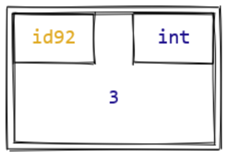
Here is a summary of the three components of a Python object.
| Object id | Object type | Object value | |
|---|---|---|---|
| Description | A unique identifier for the object. | The data type of the object. | The value of the object. |
| How to see it | Built-in id function |
Built-in type function |
Evaluate it |
| Example | |
|
|
| Can change? | No | No | Yes, for some data types |
| Unique among all objects | Yes | No | No |
You’ll note that we’ve said that an object’s value can change for some data types. You’re probably wondering which of those data types can change, but perhaps at this point you can anticipate what we’ll say next—read on to find out! 😸