Expressions in predicate logic with a single quantifier can generally be translated into English as either “there exists an element \(x\) of set \(S\) that satisfies \(P(x)\)” (existential quantifier) or “every element \(x\) of set \(S\) satisfies \(P(x)\)” (universal quantifier). However, as the kinds of data we work with grow more complex, we will often find situations where we’re dealing with multiple variables interacting with each other. So to wrap up this chapter, we’ll take a deeper look at predicate logic and investigate precisely what predicate formulas mean when they contain multiple quantified variables.
A “love”-ly example
To begin, recall our \(Loves\) predicate that we introduced in Section 3.2, which we visualized with the following diagram:
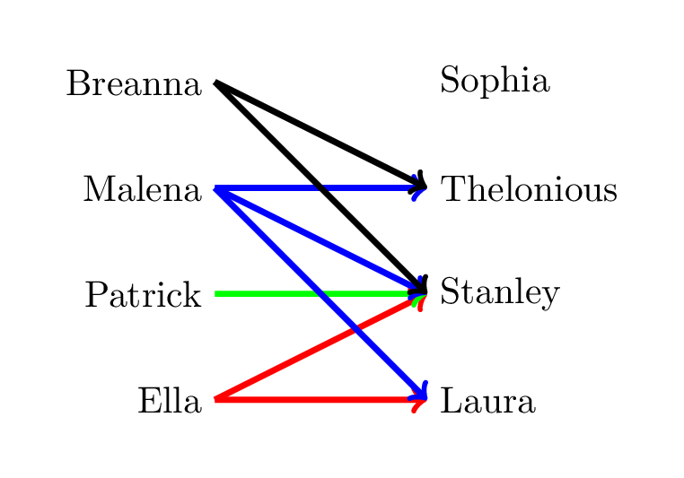
This allowed us to express statements like \(\exists a \in A,~Loves(a, \text{Thelonious})\) (which is True) and \(\forall b \in B,~Loves(\text{Malena}, b)\) (which is False).
Let’s now introduce a new way of representing the \(Loves\) predicate truth values, using a two-dimensional truth table. This is similar to the truth tables for propositional operators we used in Section 3.1, but we’re using rows and columns to distinguish between the two domains.
| Sophia | Thelonious | Stanley | Laura | |
|---|---|---|---|---|
| Breanna | False | True | True | False |
| Malena | False | True | True | True |
| Patrick | False | False | True | False |
| Ella | False | False | True | True |
In this table format, we can interpret the two above statements as follows: - \(\exists a \in A,~Loves(a, \text{Thelonious})\) means “there exists one True value in the ‘Thelonious’ column” - \(\forall b \in B,~Loves(\text{Malena}, b)\) means “all values are True in the ‘Malena’ row”
Now, multiple variables
The two statements we just looked at used just one variable (\(a \in A\) or \(b \in B\)), but what if we wanted to quantify both of the inputs to \(Loves\)? Consider the following predicate formula: \[\forall a \in A,~\forall b \in B,~Loves(a, b).\]
We translate this as “for every person \(a\) in \(A\), for every person \(b\) in \(B\), \(a\) loves \(b\)”. After some thought, we notice that the order in which we quantified \(a\) and \(b\) doesn’t matter; the statement “for every person \(b\) in \(B\), for every person \(a\) in \(A\), \(a\) loves \(b\)” means exactly the same thing! In both cases, we are considering all possible pairs of people (one from \(A\) and one from \(B\)). In the truth table above, this statement can be interpreted as “every entry is True”.
In general, when we have two consecutive universal quantifiers the order does not matter. That is, the following two formulas are equivalent:Tip: when the domains of the two variables are the same, we typically combine the quantifications, e.g., \(\forall x \in S,~ \forall y \in S,~ P(x, y)\) into \(\forall x,y \in S,~ P(x, y)\).
- \(\forall x \in S_1,~ \forall y \in S_2,~ P(x, y)\)
- \(\forall y \in S_2,~ \forall x \in S_1,~ P(x, y)\)
The same is true of two consecutive existential quantifiers. Consider the analogous formula except with \(\exists\) instead of \(\forall\):
\[\exists a \in A,~\exists b \in B,~Loves(a, b).\]
We translate this as “there exists a person \(a\) in \(A\), and there exists a person \(b\) in \(B\), where \(a\) loves \(b\)”. In the truth table above, this statement can be interpreted as “there exists a value that is True”.
The statements “there exist an \(a\) in \(A\) and \(b\) in \(B\) such that \(a\) loves \(b\)” and “there exist a \(b\) in \(B\) and \(a\) in \(A\) such that \(a\) loves \(b\).” Again, they mean the same thing: in this case, we only care about one particular pair of people (one from \(A\) and one from \(B\)), so the order in which we pick the particular \(a\) and \(b\) doesn’t matter. In general, the following two formulas are equivalent:
- \(\exists x \in S_1,~ \exists y \in S_2,~ P(x, y)\)
- \(\exists y \in S_2,~ \exists x \in S_1,~ P(x, y)\)
Alternating quantifiers
Even though consecutive quantifiers of the same type are pretty straightforward, this is not the case when we have two different quantifiers for the variables, which we call alternating quantifiers.
For example, consider this predicate formula: \[\forall a \in A,~ \exists b \in B,~ Loves(a, b).\]
This can be translated as “For every person \(a\) in \(A\), there exists a person \(b\) in \(B\), such that \(a\) loves \(b\).” Or put a bit more naturally, “For every person \(a\) in \(A\), \(a\) loves someone in \(B\),” which can be shortened even further to “Everyone in \(A\) loves someone in \(B\).” This is true: every person in \(A\) loves at least one person.
| \(a\) (from \(A\)) | \(b\) (a person in \(B\) who \(a\) loves) |
|---|---|
| Breanna | Thelonious |
| Malena | Laura |
| Patrick | Stanley |
| Ella | Stanley |
Note that the choice of person who \(a\) loves depends on \(a\): this is consistent with the latter part of the English translation, “\(a\) loves someone in \(B\).” Looking back to our truth table, we can interpret this statement as “in every row there exists a True value” (but which entry is True can be different across the different rows).
Let us contrast this with the similar-looking formula, where the order of the quantifiers has changed: \[\exists b \in B,~ \forall a \in A,~ Loves(a, b).\] This formula’s meaning is quite different: “there exists a person \(b\) in \(B\), where for every person \(a\) in \(A\), \(a\) loves \(b\).” Put more naturally, “there is a person \(b\) in \(B\) who is loved by everyone in \(A\)” or “someone in \(B\) is loved by everyone in \(A\)”. And in terms of the table, this statements means “there exists a column where every entry is True”.
For our definition of the Loves predicate, this statement happens to be True because everyone in \(A\) loves Stanley:
| \(b\) (from \(B\)) | Loved by everyone in \(A\)? |
|---|---|
| Sophia | No |
| Thelonious | No |
| Stanley | Yes |
| Laura | No |
But the statement would not be True if, for example, we removed the love connection between Malena and Stanley. In this case, Stanley would no longer be loved by everyone, and so no one in \(B\) is loved by everyone in \(A\). But notice that even if Malena no longer loves Stanley, the previous statement (“everyone in \(A\) loves someone”) remains True.
So we would have a case where switching the order of quantifiers changes the meaning of a formula! In both cases, the existential quantifier \(\exists b \in B\) involves making a choice of person from \(B\). But in the first case, this quantifier occurs after \(a\) is quantified, so the choice of \(b\) is allowed to depend on the choice of \(a\). In the second case, this quantifier occurs before \(a\), and so the choice of \(b\) must be independent of the choice of \(a\).
When reading a nested quantified expression, you should read it from left to right, and pay attention to the order of the quantifiers. In order to see if the statement is True, whenever you come across a universal quantifier, you must verify the statement for every single value that this variable can take on. Whenever you see an existential quantifier, you only need to exhibit one value for that variable such that the statement is True, and this value can depend on the variables to the left of it, but not on the variables to the right of it.
Translating multiple quantifiers into Python code
Now let’s see how we could represent this example in Python. First, recall the table of who loves whom from above:
| Sophia | Thelonious | Stanley | Laura | |
|---|---|---|---|---|
| Breanna | False | True | True | False |
| Malena | False | True | True | True |
| Patrick | False | False | True | False |
| Ella | False | False | True | True |
And we can represent this table of who loves whom in Python as a list of lists.
[
  [False, True, True, False],   # The "Breanna" row
  [False, True, True, True],    # The "Malena" row
  [False, False, True, False],  # The "Patrick" row
  [False, False, True, True]    # The "Ella" row
]
Our list is the same as the table above, except with the people’s names removed. Each row of the table represents a person from set \(A\), while each column in the table represents a person from set \(B\). We’ve kept the order the same; so the first row represents Breanna, while the third column represents Stanley.
Now, how are we going to access the data from this table? For this
section we’re going to put all of our work into a new file called
loves.py, and so we’ll start by defining a new variable in
this file:
# In loves.py
LOVES_TABLE = [
  [False, True, True, False],
  [False, True, True, True],
  [False, False, True, False],
  [False, False, True, True]
]
Note about global constants
This is the first time we’ve defined a variable within a Python file
(rather than the Python console) that is not in a function
definition. Variables defined in this way are called global
constants, to distinguish them from the local variables defined
within
functions. The term “constant” is not important right now, but
will become very important later in the course. In Python, global
constants typically use the ALL_CAPS naming convention to
distinguish them from local variables.
Global constants are called “global” because their scope is the entire Python module in which they are defined: they can be accessed anywhere in the file, including all function bodies. They can also be imported and used in other Python modules, and are available when we run the file in the Python console.
Exploring LOVES_TABLE
To start, let’s run our loves.py file in the Python
console so we can play around with the LOVES_TABLE value.
Because LOVES_TABLE is a list of lists, where each inner
list represents a row of the table, it’s easy to access a single row
with list indexing:
>>> LOVES_TABLE[0]  # This is the first row of the table
[False, True, True, False]
From here, we can access individual elements of the table, which represent an individual value of the \(Loves(a, b)\) predicate.
>>> LOVES_TABLE[0][1]  # This is the (0, 1) entry in the table
True
>>> LOVES_TABLE[2][3]  # This is the (2, 3) entry in the table
False
In general, LOVES_TABLE[i][j] evaluates to the entry in
row i and column j of the table. Finally,
since the data is stored by rows, accessing columns is a little more
work. To access column j, we can use a list comprehension
to access the j-th element in each row. Here is an example
for accessing the leftmost column (j = 0):
>>> [LOVES_TABLE[i][0] for i in range(0, 4)]
[False, False, False, False]
Now, let’s return to our Python file loves.py and define
a version of our \(Loves\) predicate.
First, we add two more constants to represent the sets \(A\) and \(B\), but using a dictionary to map names to
their corresponding indices in LOVES_TABLE.
# In loves.py
LOVES_TABLE = [
    [False, True, True, False],
    [False, True, True, True],
    [False, False, True, False],
    [False, False, True, True]
]

A = {
    'Breanna': 0,
    'Malena': 1,
    'Patrick': 2,
    'Ella': 3
}

B = {
    'Sophia': 0,
    'Thelonious': 1,
    'Stanley': 2,
    'Laura': 3,
}
Next, we define a loves predicate, which takes in two
strings and returns whether person a loves person
b. Note that because this function is defined in the same
file as LOVES_TABLE, it can access that global constant in
its body.
def loves(a: str, b: str) -> bool:
    """Return whether person a loves person b.

    Assuming that:
      - a in A
      - b in B

    >>> loves('Breanna', 'Sophia')
    False
    """
    a_index = A[a]
    b_index = B[b]
    return LOVES_TABLE[a_index][b_index]
Now that we’ve seen how to access individual entries, rows, and columns from the table, let’s turn to how we would represent the statements in predicate logic we’ve written in this section. First, we can express \(\forall a \in A,~ \forall b \in B,~ Loves(a, b)\) as the expression:
>>> all({loves(a, b) for a in A for b in B})
False
And similarly, we can express \(\exists a \in A,~ \exists b \in B,~ Loves(a, b)\) as the expression:
>>> any({loves(a, b) for a in A for b in B})
True
These two examples illustrate how Python’s all and
any functions naturally enable us to express multiple
quantifiers of the same type. But what about the expressions we looked
at with alternating quantifiers? Consider \(\forall a \in A,~ \exists b \in B,~ Loves(a,
b)\). It is possible to construct a nested expression that
represents this one as well:
>>> all({any({loves(a, b) for b in B}) for a in A})
True
Though this Python expression is structurally equivalent to the
statement in predicate logic, it’s longer and a bit harder to read. In
general we try to avoid lots of expression nesting in programming, and a
rule of thumb we’ll try to follow in this course is to avoid nesting
all/any calls. Instead, we can pull out
the inner any into its own function, which not only reduces
the nesting but makes it clearer what’s going on:
def loves_someone(a: str) -> bool:
    """Return whether a loves at least one person in B.

    Assuming that:
      - a in A
    """
    return any({loves(a, b) for b in B})


>>> all({loves_someone(a) for a in A})
True
Similarly, we can express the statement \(\exists b \in B,~ \forall a \in A,~
Loves(a,b)\) in two different ways. With a nested
any/all:
>>> any({all({loves(a, b) for a in A}) for b in B})
True
And by pulling out the inner all expression into a named
function:
def loved_by_everyone(b: str) -> bool:
    """Return whether b is loved by everyone in A.

    Assuming that:
      - b in B
    """
    return all({loves(a, b)} for a in A)


>>> any({loved_by_everyone(b) for b in B})
True
And for your reference, here is our final loves.py
file:
# In loves.py
LOVES_TABLE = [
    [False, True, True, False],
    [False, True, True, True],
    [False, False, True, False],
    [False, False, True, True]
]

A = {
    'Breanna': 0,
    'Malena': 1,
    'Patrick': 2,
    'Ella': 3
}

B = {
    'Sophia': 0,
    'Thelonious': 1,
    'Stanley': 2,
    'Laura': 3,
}

def loves(a: str, b: str) -> bool:
    """Return whether a loves at least one person in B.

    Assuming that:
      - a in A
      - b in B

    >>> loves('Breanna', 'Sophia')
    False
    """
    a_index = A[a]
    b_index = B[b]
    return LOVES_TABLE[a_index][b_index]


def loves_someone(a: str) -> bool:
    """Return whether a loves at least one person in B.

    Assuming that:
      - a in A
    """
    return any({loves(a, b) for b in B})


def loved_by_everyone(b: str) -> bool:
    """Return whether b is loved by everyone in A.

    Assuming that:
      - b in B
    """
    return all({loves(a, b) for a in A})
Looking ahead
In this section, we’ve introduced the notion of lists within lists to represent truth tables for binary predicates. In Chapter 5, we’ll study tabular data more generally, as well as other forms of nested collections of data. We’ll see how these more complex data structures can be used to represent real-world data for our programs.